Torch Forecasting Models#
This document was written for darts version 0.15.0 and later.
We assume that you already know about covariates in Darts. If you’re new to the topic we recommend you to read our guide on covariates first.
Content of this guide#
Introduction section covers the most important points about Torch Forecasting Models (TFMs):
Input data usage section gives an in-depth guide of how input data is used when training and predicting with TFMs:
Advanced functionalities section provides some example of TFMs advanced features:
Performance optimization section lists tricks to speed up the computation during training.
Introduction#
In Darts, Torch Forecasting Models (TFMs) are broadly speaking “machine learning based” models, which denote PyTorch-based (deep learning) models.
TFMs train and predict on fixed-length chunks (sub-samples) of your input target and *_covariates series (if supported). Target is the series for which we want to predict the future, *_covariates are the past and / or future covariates.
Each chunk contains an input chunk - representing the sample’s past - and an output chunk - the sample’s future. The sample’s prediction point lies at the end of the input chunk. The length of these chunks has to be specified at model creation with parameters input_chunk_length and output_chunk_length (more on chunks in the next subsection).
# model that looks 7 time steps back (past) and 1 time step ahead (future)
model = SomeTorchForecastingModel(input_chunk_length=7,
                                  output_chunk_length=1,
                                  **model_kwargs)
All TFMs can be trained on single or multiple target series and, depending on their covariate support (covered in this subsection on covariates support), past_covariates and / or future_covariates. When using covariates you have to supply one dedicated past and / or future covariates series for each target series.
Optionally, you can use a validation set with dedicated covariates during training. If the covariates have the required time spans, you can use the same for training, validation and prediction. (covered in this subsection on time span requirements)
# fit the model on a single target series with optional past and / or future covariates
model.fit(target,
          past_covariates=past_covariates,
          future_covariates=future_covariates,
          val_series=target_val,  # optionally, use a validation set
          val_past_covariates=past_covariates_val,
          val_future_covariates=future_covariates_val)

# fit the model on multiple target series
model.fit([target, target2, ...],
          past_covariates=[past_covariates, past_covariates2, ...],
          ...
          )
You can produce forecasts for any input target TimeSeries or for several targets given as a sequence of TimeSeries. This will also work on series that have not been seen during training, as long as each series contains at least input_chunk_length time steps.
# predict the next n=3 time steps for any input series with `series`
prediction = model.predict(n=3,
                           series=target,
                           past_covariates=past_covariates,
                           future_covariates=future_covariates)
If you want to know more about the training and prediction process of our Torch Forecasting Models and how they work with covariates, read on.
Top level look at training and predicting with chunks#
In Figure 1 you can see how your data is distributed to the input and output chunks for each sample when calling fit() or predict(). For this example we look at data with daily frequency. The input chunk extracts values from target and optionally from past_covariates and / or future_covariates that fall into the input chunk time span. These “past” values of future_covariates are called “historic future covariates”.
The output chunk only takes optional future_covariates values that fall into the output chunk time span. The future values of our past_covariates - “future past covariates” - are only used to provide the input chunk of upcoming samples with new data.
All this information is used to predict the “future target” - the next output_chunk_length points after the end of “past target”.
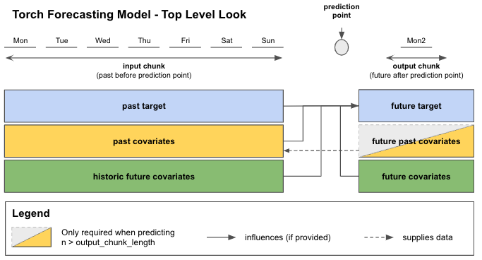
Figure 1: Top level look at training / predicting on chunks with Torch Forecasting Models
When calling predict() and depending on your forecast horizon n, the model can either predict in one go (if n <= output_chunk_length), or auto-regressively, by predicting on multiple chunks in the future (if n > output_chunk_length). That is the reason why when predicting with past_covariates you might have to supply additional “future values of your past_covariates”.
Torch Forecasting Model Covariates Support#
Under the hood, Darts has 5 types of {X}CovariatesModel classes implemented to cover different combinations of the covariate types mentioned before:
Class |
past covariates |
future past covariates |
future covariates |
historic future covariates |
|---|---|---|---|---|
|
✅ |
✅ |
||
|
✅ |
|||
|
✅ |
✅ |
||
|
✅ |
✅ |
✅ |
|
|
✅ |
✅ |
✅ |
✅ |
Table 1: Darts’ “{X}CovariatesModels” covariate support
Each Torch Forecasting Model inherits from one {X}CovariatesModel (covariate class names are abbreviated by the X-part):
TFM |
|
|
|
|
|
|---|---|---|---|---|---|
|
✅ |
||||
|
✅ |
||||
|
✅ |
||||
|
✅ |
||||
|
✅ |
||||
|
✅ |
||||
|
✅ |
||||
|
✅ |
||||
|
✅ |
||||
|
✅ |
Table 2: Darts’ Torch Forecasting Model covariate support
Required target time spans for training, validation and prediction#
The relevant data is extracted automatically by the models, based on the time axes of the series.
You can use the same covariates series for both fit() and predict() if they meet the requirements below.
Training only works if at least one sample with an input and output chunk can be extracted from the data you passed to fit(). This applies both to training and validation data. In terms of minimum required time spans, this means:
targetseries of minimum lengthinput_chunk_length + output_chunk_length*_covariatestime span requirements forfit()from covariates guide section 2.3.
For prediction you have to supply the target series that you wish to forecast. For any forecast horizon n the minimum time span requirements are:
targetseries of minimum lengthinput_chunk_length*_covariatestime span requirements forpredict()also from from covariates guide section 2.3.
Side note: Our *RNNModels accept a training_length parameter at model creation instead of output_chunk_length. Internally the output_chunk_length for these models is automatically set to 1. For training, past target must have a minimum length of training_length + 1 and for prediction, a length of input_chunk_length.
In-depth look at how input data is used when training and predicting with TFMs#
Training#
Let’s have a look at how the models work under the hood.
Let’s assume we run an ice-cream shop and we want to predict sales for the next day. We have one year (365 days) past data of our end-of-day ice-cream sales and of the average measured daily ambient temperature. We also noticed that our ice-cream sales depend on the day of the week so we want to include this in our model.
past target: actual past ice-cream sales
ice_cream_salesfuture target: predict the ice-cream sales for the next day
past covariates: measured average daily temperatures in the past
temperaturefuture covariates: day of the week for past and future
weekday
Checking Table 1, a model that would accommodate this kind of covariates would be a
SplitCovariatesModel (if we don’t use historic values of future covariates), or
MixedCovariatesModel (if we do). We choose a MixedCovariatesModel - the TFTModel.
Imagine that we saw a pattern in our past ice cream sales that repeated week after week.
So we set input_chunk_length = 7 days to let the model look back an entire week into the past.
The output_chunk_length can be set to 1 day to predict the next day.
Now we can create a model and train it! Figure 2 shows you how TFTModel will use our data.
from darts.models import TFTModel

model = TFTModel(input_chunk_length=7, output_chunk_length=1)
model.fit(series=ice_cream_sales,
          past_covariates=temperature,
          future_covariates=weekday)
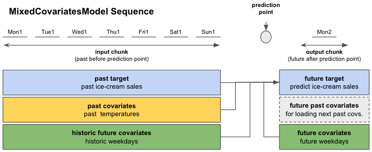
Figure 2: Overview of a single sequence from our ice-cream sales example; Mon1 - Sun1 stand for the first 7 days from our training dataset (week 1 of the year). Mon2 is the Monday of week 2.
When calling fit(), the models will build an appropriate darts.utils.data.TorchTrainingDataset, which specifies how to slice the data to obtain training samples. If you want to control this slicing yourself, you can instantiate your own TorchTrainingDataset and call model.fit_from_dataset() instead of fit(). By default, most models (though not all) will build sequential datasets, which basically means that all sub-slices of length input_chunk_length + output_chunk_length in the provided series will be used for training.
So during training, the torch models will go through the training data in sequences (see Figure 3). Using information from the input chunk and output chunk, the model predicts the future target on the output chunk. The training loss is evaluated between the predicted future target and the actual target value on the output chunk. The model trains itself by minimizing the loss over all sequences.
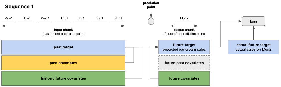
Figure 3: Prediction and loss evaluation in a single sequence
After having completed computations on the first sequence, the model moves to the next one and performs the same training steps. The starting point of each sequence is selected randomly from the sequential dataset. Figure 4 shows how this would look like if by pure chance the second sequence started one time step (day) after the first.
This sequence-to-sequence process is repeated until all 365 days were covered.
Side note: Having “long” target series can result in a very large number of training sequences / samples. You can set an upper bound for the number of sequences / samples per target that the model should be trained on with fit()-parameter max_samples_per_ts. This will take the most recent sequences for every target series (sequences closest to target end).
# fit only on the 10 "most recent" sequences
model.fit(target, max_samples_per_ts=10)
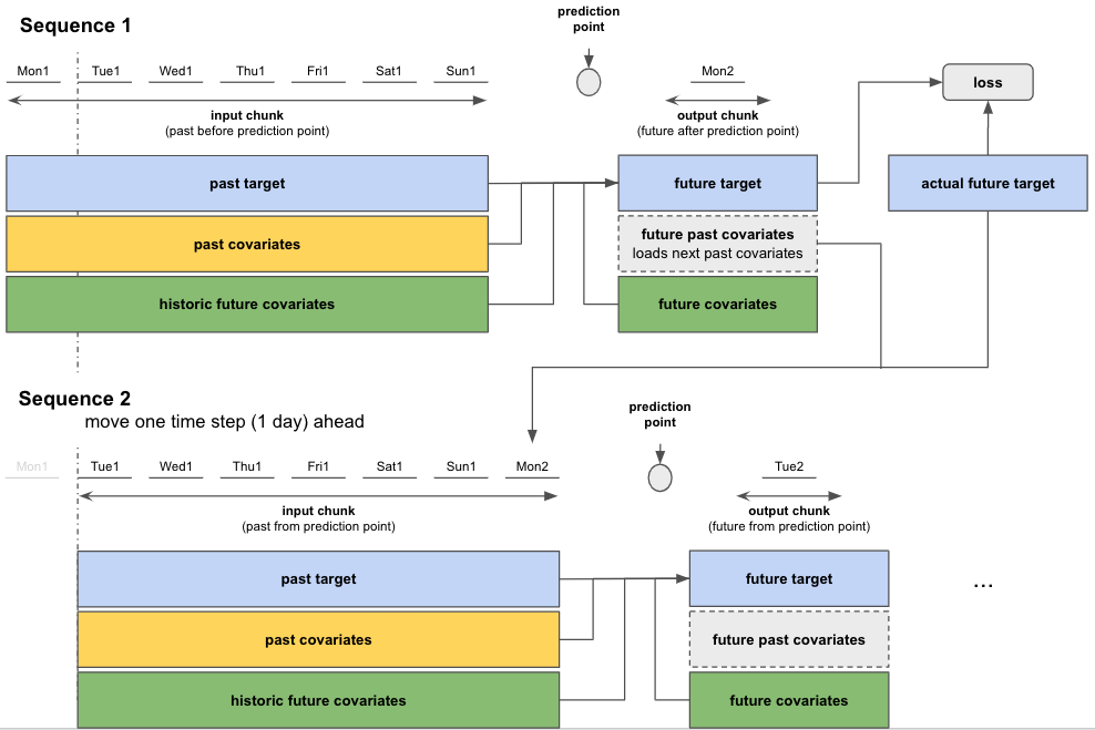
Figure 4: Sequence-to-sequence: Move to next sequence and repeat training steps
Training with a validation dataset#
You can also train your models with a validation dataset:
# create train and validation sets
ice_cream_sales_train, ice_cream_sales_val = ice_cream_sales.split_after(training_cutoff)

# train with validation set
model.fit(series=ice_cream_sales_train,
          past_covariates=temperature,
          future_covariates=weekday,
          val_series=ice_cream_sales_val,
          val_past_covariates=temperature,
          val_future_covariates=weekday)
If you split your data, you have to define a training_cutoff (a date or fraction at which to split the dataset) so that both the train and validation datasets satisfy the minimum length requirements
from this subsection on time span requirements
Instead of splitting by time, you can also use another subset of time series as validation set.
The model trains itself the same way as before but additionally evaluates the loss on the validation dataset. If you want to keep track of the best performing model on the validation set, you have to enable checkpoint saving as shown next.
Forecasting#
After having trained the model, we want to predict the future ice-cream sales for any number of days after our 365 days training data.
The actual prediction works very similar to how we trained the data on sequences. Depending on the number of days we want to predict - the forecast horizon n - we distinguish between two cases:
If
n <= output_chunk_length: we can predictnin one go (using one “internal model call”)in our example: predict the next day’s ice-cream sales (
n = 1)
If
n > output_chunk_length: we must predictnby calling the internal model multiple times. Each call outputsoutput_chunk_lengthprediction points. We go through as many calls as needed until we get to the finalnprediction points, in an auto-regressive fashion.in our example: predict ice-cream sales for the next 3 days at once (
n = 3)
To do this we have to supply additional
past_covariatesfor the nextn - output_chunk_length = 2time steps (days) after the end of our 365 days training data. Unfortunately, we do not have measuredtemperaturefor the future. But let’s assume we have access to temperature forecasts for the next 2 days. We can just append them totemperatureand the prediction will work!temperature = temperature.concatenate(temperature_forecast, axis=0)
prediction = model.predict(n=n,
                           series=ice_cream_sales_train,
                           past_covariates=temperature,
                           future_covariates=weekday)
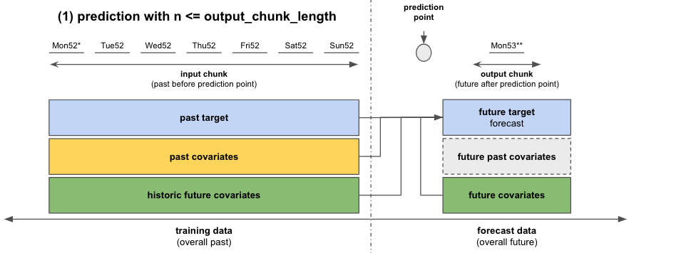
Figure 5: Forecast with a single sequence for n <= output_chunk_length
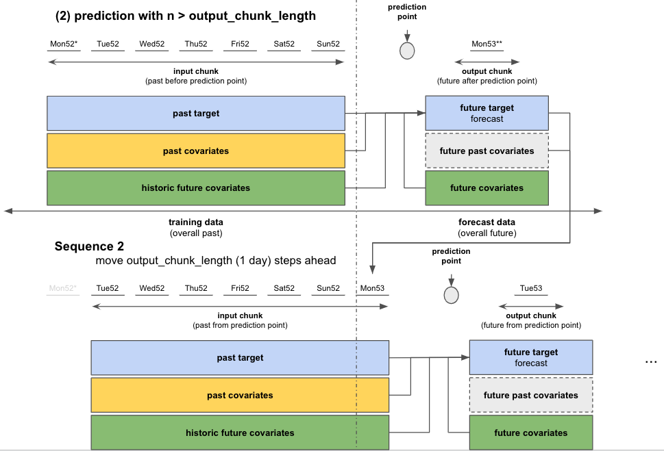
Figure 6: Auto-regressive forecast for n > output_chunk_length
Advanced Functionnalities#
Saving and Loading Model States#
❗ Warning ❗ At this stage of Darts development, we are not (yet) ensuring backward compatibility, so it might not always be possible to load a model saved by an older version of the library.
For models trained on GPU with versions of Darts <= 0.22.0 that need to be loaded on CPU with a version of Darts >= 0.23.0, please look at the code snipped provided in this issue.
Automatic checkpointing#
Automic checkpointing during training allows you to:
keep track of the model state over the latest 5 epochs, and the best performing epoch based on the validation set loss
load a model from checkpoint to resume training in case it was interrupted
load a model from checkpoint for inference / forecasting
You can activate checkpointing at model creation:
model = SomeTorchForecastingModel(..., model_name='my_model', save_checkpoints=True)

# checkpoints are saved automatically
model.fit(...)

# load the model state that performed best on validation set
best_model = model.load_from_checkpoint(model_name='my_model', best=True)
Manual saving and loading#
You can also manually save the model at its current state and load it:
model.save("/your/path/to/save/model.pt")
loaded_model = model.load("/your/path/to/save/model.pt")
Training and saving on GPU, loading on CPU#
You can load a model to CPU that was trained and saved on GPU (see detailed documentation):
# define a model using gpu as accelerator
model = SomeTorchForecastingModel(...,
                                  model_name='my_model',
                                  save_checkpoints=True,
                                  pl_trainer_kwargs={
                                                     "accelerator":"gpu",
                                                     "devices": -1,
                                                     })

# train the model, automatic checkpoints will be created
model.fit(...)

# specify the device to which the model should be loaded
loaded_model = SomeTorchForecastingModel.load_from_checkpoint(model_name='my_model',
                                                              best=True,
                                                              map_location="cpu")
loaded_model.to_cpu()

# run inference
loaded_model.predict(...)
Manual saves can also be loaded to CPU:
model.save("/your/path/to/save/model.pt")
loaded_model = model.load("/your/path/to/save/model.pt", map_location="cpu")
loaded_model.to_cpu()
Retraining or finetuning a pretrained model#
To re-train or fine-tune a model using a different optimizer and/or learning rate scheduler, you can load the weights from the automatic checkpoints into a new model:
# model with identical architecture but different optimizer (default: torch.optim.Adam)
model_finetune = SomeTorchForecastingModel(...,  # use identical parameters & values as in original model
                                           optimizer_cls=torch.optim.SGD,
                                           optimizer_kwargs={"lr": 0.001})

# load the weights from a checkpoint
model_finetune.load_weights_from_checkpoint(model_name='my_model', best=True)

model_finetune.fit(...)
and similarly for manual saves and the learning rate scheduler:
# model with identical architecture but different lr scheduler (default: None)
model_finetune = SomeTorchForecastingModel(...,  # use identical parameters & values as in original model
                                           lr_scheduler_cls=torch.optim.lr_scheduler.ExponentialLR,
                                           lr_scheduler_kwargs={"gamma": 0.09})

# load the weights from a manual save
model_finetune.load_weights("/your/path/to/save/model.pt")
Additionally, all TorchForecastingModel (including FoundationModel) support fine-tuning through the enable_finetuning parameter. This allows you to freeze or unfreeze specific model parameters for transfer learning:
# full fine-tuning: all parameters are trainable
model = SomeTorchForecastingModel(..., enable_finetuning=True)

# partial fine-tuning: freeze specific layers
model = SomeTorchForecastingModel(..., enable_finetuning={"freeze": ["layer.pattern.*"]})

# partial fine-tuning: only unfreeze specific layers
model = SomeTorchForecastingModel(..., enable_finetuning={"unfreeze": ["layer.pattern.*"]})

# optionally, load pre-trained weights (not required for foundation models)
model.load_weights("/your/path/to/save/model.pt")

# fine-tune
model.fit(...)
For a comprehensive walkthrough of fine-tuning Torch Forecasting Models and Foundation Models, check out the Fine-Tuning example notebook.
Exporting model to ONNX format for inference#
It is also possible to export the model weights to the ONNX format to run inference in a lightweight environment. The example below works for any TorchForecastingModel except RNNModel and for optional usage of past, future and / or static covariates. Note that all series and covariates must extend far enough into the past (input_chunk_length) and future (output_chunk_length) relative to the end of the target series. It will not be possible to forecast a horizon n > output_chunk_length without implementing the auto-regression logic.
model = SomeTorchForecastingModel(...)
model.fit(...)

# make sure to have `onnx` and `onnxruntime` installed
onnx_filename = "example_onnx.onnx"
model.to_onnx(onnx_filename, export_params=True)
Now, to load the model and predict steps after the end of the series:
from typing import Optional
import onnx
import onnxruntime as ort
import numpy as np
from darts import TimeSeries
from darts.utils.onnx_utils.py import prepare_onnx_inputs

onnx_model = onnx.load(onnx_filename)
onnx.checker.check_model(onnx_model)
ort_session = ort.InferenceSession(onnx_filename)

# use helper function to extract the features from the series
past_feats, future_feats, static_feats = prepare_onnx_inputs(
    model=model,
    series=series,
    past_covariates=ts_past,
    future_covariates=ts_future,
)

# extract only the features expected by the model
ort_inputs = {}
for name, arr in zip(['x_past', 'x_future', 'x_static'], [past_feats, future_feats, static_feats]):
    if name in [inp.name for inp in list(ort_session.get_inputs())]:
        ort_inputs[name] = arr

# output has shape (batch, output_chunk_length, n components, 1 or n likelihood params)
ort_out = ort_session.run(None, ort_inputs)
Callbacks#
Callbacks are a powerful way to monitor or control the behavior of the model during the training process. Some examples:
Performance Monitoring: compute additional metrics (in addition of the default losses)
Early stopping: stop the training once the model has converged
…
With callbacks you can add custom code to an existing process at predefined points / hooks. The code is triggered once the process execution reaches the corresponding hooks. Some example hooks:
beginning / end of training
beginning / end of train / validation step
…
Some useful predefined PyTorch Lightning callbacks can be found here.
Example with Early Stopping#
Early stopping is an efficient way to avoid overfitting and reduce training time. It will exit the training process once the validation loss has not significantly improved over some epochs.
You can use Early Stopping with any TorchForecastingModel, leveraging PyTorch Lightning’s EarlyStopping callback:
import pandas as pd
from pytorch_lightning.callbacks import EarlyStopping
from torchmetrics import MeanAbsolutePercentageError

from darts.dataprocessing.transformers import Scaler
from darts.datasets import AirPassengersDataset
from darts.models import NBEATSModel

# read data
series = AirPassengersDataset().load()

# create training and validation sets:
train, val = series.split_after(pd.Timestamp(year=1957, month=12, day=1))

# normalize the time series
transformer = Scaler()
train = transformer.fit_transform(train)
val = transformer.transform(val)

# any TorchMetric or val_loss can be used as the monitor
torch_metrics = MeanAbsolutePercentageError()

# early stop callback
my_stopper = EarlyStopping(
    monitor="val_MeanAbsolutePercentageError",  # "val_loss",
    patience=5,
    min_delta=0.05,
    mode='min',
)
pl_trainer_kwargs = {"callbacks": [my_stopper]}

# create the model
model = NBEATSModel(
    input_chunk_length=24,
    output_chunk_length=12,
    n_epochs=500,
    torch_metrics=torch_metrics,
    pl_trainer_kwargs=pl_trainer_kwargs)

# use validation set for early stopping
model.fit(
    series=train,
    val_series=val,
)
To use early-stopping and pruning in the context of hyperparameter optimization, check out this guide.
Example of custom callback to store losses#
Training and validation loss can be automatically logged with tensorboard. When activated, Darts will by default store the logs to a folder darts_logs in the current working directory. You can change this with model parameters work_dir, and model_name.
model = SomeTorchForecastingModel(..., log_tensorboad, save_checkpoints=True)
model.fit(...)
After installing the tensorboard library, you can visualize the logs from the command line:
tensorboad --log_dir darts_logs
Let’s check out how to implement a custom callback to make the model losses accessible in Python.
from pytorch_lightning.callbacks import Callback

class LossLogger(Callback):
    def __init__(self):
        self.train_loss = []
        self.val_loss = []

    # will automatically be called at the end of each epoch
    def on_train_epoch_end(self, trainer: "pl.Trainer", pl_module: "pl.LightningModule") -> None:
        self.train_loss.append(float(trainer.callback_metrics["train_loss"]))

    def on_validation_epoch_end(self, trainer: "pl.Trainer", pl_module: "pl.LightningModule") -> None:
        self.val_loss.append(float(trainer.callback_metrics["val_loss"]))


loss_logger = LossLogger()

model = SomeTorchForecastingModel(
    ...,
    nr_epochs_val_period=1,  # perform validation after every epoch
    pl_trainer_kwargs={"callbacks": [loss_logger]}
)

# fit must include validation set for "val_loss"
model.fit(...)
Note : The callback will give one more element in the loss_logger.val_loss as the model trainer performs a validation sanity check before the training begins.
Performance Recommendations#
This section recaps the main factors impacting the performance when training and using torch-based models.
Build your TimeSeries using 32-bits data#
The models in Darts will dynamically cast themselves (to 64 or 32-bits)
to follow the dtype in the TimeSeries. Large performance and memory gains
can often be obtained when everything (data and model) is in float32.
To achieve this, it is enough to build your TimeSeries from arrays (or Dataframe-backing array) having dtype np.float32, or simply call my_series32 = my_series.astype(np.float32). Calling my_series.dtype gives you the dtype of your TimeSeries.
Use a GPU#
In many cases using a GPU will provide a drastic speedup compared to CPU. It can also incur some overheads (for transferring data to/from the GPU), so some testing and tuning is often necessary. We refer to our GPU/TPU guide for more information on how to setup a GPU (or a TPU) via PyTorch Lightning.
Tune the batch size#
A larger batch size tends to speed up the training because it reduces the number of backward passes per epoch and has the potential to better parallelize computation. However it also changes the training dynamics (e.g. you might need more epochs, and the convergence dynamics is affected). Furthermore larger batch sizes increase memory consumption. So here too some testing is required.
Tune num_loader_workers#
All deep learning models in Darts have a parameter dataloader_kwargs in their fit() and predict() functions, which configures the PyTorch DataLoaders. The num_workers parameter for PyTorch DataLoaders can be set using the num_workers key in the dataloader_kwargs dictionary.
Setting num_workers > 0 will use additional workers to load the data. This typically incurs some overhead (notably increasing memory consumption), but in some cases it can also substantially improve performance.
The ideal value depends on many factors such as the batch size, whether you are using a GPU, the number of CPU cores available, and whether
loading the data involved I/O operations (if the series are stored on disk).
Small models first#
Of course one of the main factors affecting performance is the model size (number of parameters) and the number of operations required by forward/backward passes. Models in Darts can be tuned (e.g. number of layers, attention heads, widths etc), and these hyper-parameters tend to have a large impact on performance. When starting out, it is a good idea to build models of modest size first.
Data in Memory and I/O bottlenecks#
It’s helpful to load all your TimeSeries in memory upfront if you can.
Darts offers the possibility to train models on any Sequence[TimeSeries],
which means that for big datasets, you can write your own Sequence implementation, and read the time series lazily from disk. This will typically incur a high I/O cost, though. So when training on multiple series, first try to build a simple List[TimeSeries] upfront, and see if it holds in the computer memory.
Do not use all possible sub-series for training#
By default, when calling fit(), the models in Darts will build a TorchTrainingDataset instance that is
suitable for the model that you are using (e.g., PastCovariatesTorchModel, FutureCovariatesTorchModel, etc.).
By default, these training datasets will often contain all possible consecutive (input, output) subseries present
in each TimeSeries. If your TimeSeries are long, this can result in a large amount of training samples, which directly (linearly)
impacts the time required to train the model for one epoch. You have two options to limit this:
Specify some
max_samples_per_tsargument to thefit()function. This will use only the most recentmax_samples_per_tssamples perTimeSeriesfor training.If this option does not do what you want, you can implement your own
TorchTrainingDatasetinstance, and define how to slice yourTimeSeriesfor training yourself. We suggest to have a look at this submodule to see examples of how to do it.
Example Benchmark#
As an example, we show here the time required to train one epoch on the first 80% of the energy dataset (darts.datasets.EnergyDataset), which consists of one multivariate series that is 28050 timesteps long and has 28 dimensions.
We train two models; NBEATSModel and TFTModel, with default parameters and input_chunk_length=48 and output_chunk_length=12 (which results in 27991 training samples with default sequential training datasets). For the TFT model, we also set the parameter add_cyclic_encoder='hour'. The tests are made on a Intel CPU i9-10900K CPU @ 3.70GHz, with an Nvidia RTX 2080s GPU, 32 GB of RAM. All TimeSeries are pre-loaded in memory and given to the models as a list.
Model |
Dataset |
dtype |
CUDA |
Batch size |
num workers |
time per epoch |
|---|---|---|---|---|---|---|
|
Energy |
64 |
no |
32 |
0 |
283s |
|
Energy |
64 |
no |
32 |
2 |
285s |
|
Energy |
64 |
no |
32 |
4 |
282s |
|
Energy |
64 |
no |
1024 |
0 |
58s |
|
Energy |
64 |
no |
1024 |
2 |
57s |
|
Energy |
64 |
no |
1024 |
4 |
58s |
|
Energy |
64 |
yes |
32 |
0 |
63s |
|
Energy |
64 |
yes |
32 |
2 |
62s |
|
Energy |
64 |
yes |
1024 |
0 |
13.3s |
|
Energy |
64 |
yes |
1024 |
2 |
12.1s |
|
Energy |
64 |
yes |
1024 |
4 |
12.3s |
|
Energy |
32 |
no |
32 |
0 |
117s |
|
Energy |
32 |
no |
32 |
2 |
115s |
|
Energy |
32 |
no |
32 |
4 |
117s |
|
Energy |
32 |
no |
1024 |
0 |
28.4s |
|
Energy |
32 |
no |
1024 |
2 |
27.4s |
|
Energy |
32 |
no |
1024 |
4 |
27.5s |
|
Energy |
32 |
yes |
32 |
0 |
41.5s |
|
Energy |
32 |
yes |
32 |
2 |
40.6s |
|
Energy |
32 |
yes |
1024 |
0 |
2.8s |
|
Energy |
32 |
yes |
1024 |
2 |
1.65 |
|
Energy |
32 |
yes |
1024 |
4 |
1.8s |
|
Energy |
64 |
no |
32 |
0 |
78s |
|
Energy |
64 |
no |
32 |
2 |
72s |
|
Energy |
64 |
no |
32 |
4 |
72s |
|
Energy |
64 |
no |
1024 |
0 |
46s |
|
Energy |
64 |
no |
1024 |
2 |
38s |
|
Energy |
64 |
no |
1024 |
4 |
39s |
|
Energy |
64 |
yes |
32 |
0 |
125s |
|
Energy |
64 |
yes |
32 |
2 |
115s |
|
Energy |
64 |
yes |
1024 |
0 |
59s |
|
Energy |
64 |
yes |
1024 |
2 |
50s |
|
Energy |
64 |
yes |
1024 |
4 |
50s |
|
Energy |
32 |
no |
32 |
0 |
70s |
|
Energy |
32 |
no |
32 |
2 |
62.6s |
|
Energy |
32 |
no |
32 |
4 |
63.6 |
|
Energy |
32 |
no |
1024 |
0 |
31.9s |
|
Energy |
32 |
no |
1024 |
2 |
45s |
|
Energy |
32 |
no |
1024 |
4 |
44s |
|
Energy |
32 |
yes |
32 |
0 |
73s |
|
Energy |
32 |
yes |
32 |
2 |
58s |
|
Energy |
32 |
yes |
1024 |
0 |
41s |
|
Energy |
32 |
yes |
1024 |
2 |
31s |
|
Energy |
32 |
yes |
1024 |
4 |
31s |