Quickstart#
In this notebook, we go over the main functionalities of the library:
We will only show some minimal “get started” examples here. For more in depth information, you can refer to our user guide and example notebooks.
Installing Darts#
We recommend using some virtual environment. Then there are mainly two ways.
With pip:
pip install darts
With conda
conda install -c conda-forge -c pytorch u8darts-all
Consult the detailed install guide if you run into issues or want to install a different flavour (avoiding certain dependencies).
First, let’s import a few things:
[1]:
# fix python path if working locally
from utils import fix_pythonpath_if_working_locally

fix_pythonpath_if_working_locally()

import warnings

warnings.filterwarnings("ignore", category=FutureWarning)
[2]:
%matplotlib inline

import matplotlib.pyplot as plt
import numpy as np
import pandas as pd
[ ]:
# use darts plotting style
from darts import set_option

set_option("plotting.use_darts_style", True)
Building and manipulating TimeSeries#
TimeSeries is the main data class in Darts. A TimeSeries represents a univariate or multivariate time series, with a proper time index. The time index can either be of type pandas.DatetimeIndex (containing datetimes), or of type pandas.RangeIndex (containing integers useful for representing sequential data without specific timestamps). In some cases, TimeSeries can even represent probabilistic series, in order for instance to obtain confidence intervals. All models in Darts
consume TimeSeries and produce TimeSeries.
Read data and build a TimeSeries#
TimeSeries can be built easily using a few factory methods:
From a
DataFrame, usingTimeSeries.from_dataframe()(docs). We support multiple frame backends such aspandas.DataFrame,polars.DataFrame,pyarrow.tableand more (see (a)).From a time index and an array of corresponding values, using
TimeSeries.from_times_and_values()(docs).From a NumPy array of values, using
TimeSeries.from_values()(docs).From a
Series, usingTimeSeries.from_series()(docs). Also here we support multiple series backends such aspandas.Series,polars.Series, and more (see (a)).Extract multiple
TimeSeriesby groups from a PandasDataFrame, usingTimeSeries.from_group_dataframe()(docs).From an
xarray.DataArray, usingTimeSeries.from_xarray()(docs).From a CSV file, using
TimeSeries.from_csv()(docs).From a JSON file, using
TimeSeries.from_json()(docs).Or use one of our built-in
TimeSeriesgeneration functions (docs).
(a) We leverage narwhals as the compatibility layer between DataFrame and Series libraries. See the narwhals documentation for all supported backends.
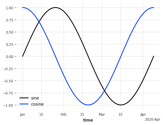
Let’s create a multivariate (two-column) TimeSeries from a DataFrame. The frame contains a sine and cosine series, and has a time index of daily frequency.
[3]:
from darts import TimeSeries
from darts.utils.utils import generate_index

# generate a sine and cosine wave
x = np.linspace(0, 2 * np.pi, 100)
sine_vals = np.sin(x)
cosine_vals = np.cos(x)

# generate a DatetimeIndex with daily frequency
dates = generate_index("2020-01-01", length=len(x), freq="D")

# create a DataFrame; here we use pandas but you can use any other backend (e.g. polars, pyarrow, ...).
df = pd.DataFrame({"sine": sine_vals, "cosine": cosine_vals, "time": dates})

series = TimeSeries.from_dataframe(df, time_col="time")
series.plot();
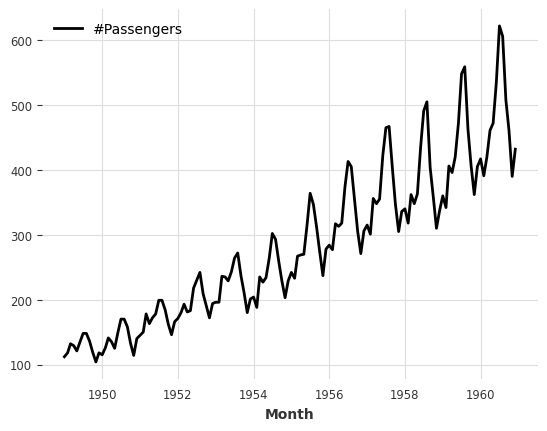
Load one of our existing datasets#
Alternatively, you can load one of our existing datasets (docs).
Below, we get a TimeSeries by directly loading the air passengers series dataset.
[4]:
from darts.datasets import AirPassengersDataset

series = AirPassengersDataset().load()
series.plot();
Export a TimeSeries#
TimeSeries can be exported in many different ways:
To a
DataFrame, usingTimeSeries.to_dataframe()(docs). We support multiple frame backends such aspandas,polars,pyarrowand more (see (a) from above).To a NumPy array of values, using
TimeSeries.values()(docs) orTimeSeries.all_values()(docs).To a
Series, usingTimeSeries.to_series()(docs). Also here we support multiple series backends (see (a) from above).To a
xarray.DataArray, usingTimeSeries.data_array()(docs).To a CSV file, using
TimeSeries.to_csv()(docs).To a JSON file, using
TimeSeries.to_json()(docs).And more!
Here an example of how to export to a polars.DataFrame. Polars is an optional dependency, so make sure to install it first (see the installation guide here)
[5]:
series[-5:].to_dataframe(backend="polars", time_as_index=False)
[5]:
| Month | #Passengers |
|---|---|
| datetime[ns] | f64 |
| 1960-08-01 00:00:00 | 606.0 |
| 1960-09-01 00:00:00 | 508.0 |
| 1960-10-01 00:00:00 | 461.0 |
| 1960-11-01 00:00:00 | 390.0 |
| 1960-12-01 00:00:00 | 432.0 |
Some TimeSeries Operations#
TimeSeries support different kinds of operations - here are a few examples.
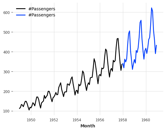
Splitting
We can also split at a fraction of the series, at a pandas Timestamp or at an integer index value.
[6]:
series1, series2 = series.split_after(0.75)
series1.plot()
series2.plot();

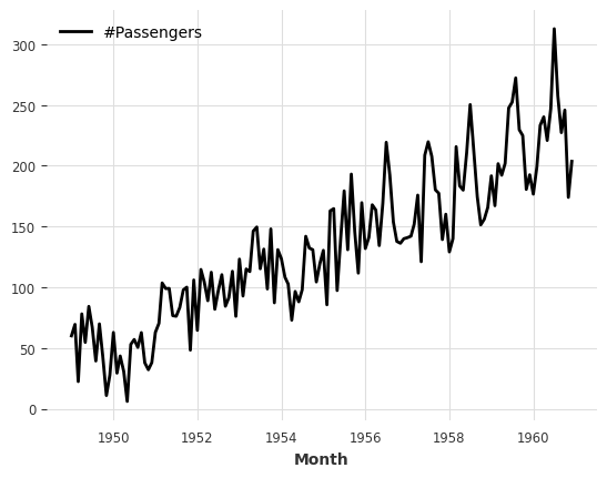
Slicing:
[7]:
series1, series2 = series[:-36], series[-36:]
series1.plot()
series2.plot();
Arithmetic operations:
[8]:
series_noise = TimeSeries.from_times_and_values(
series.time_index, np.random.randn(len(series))
)
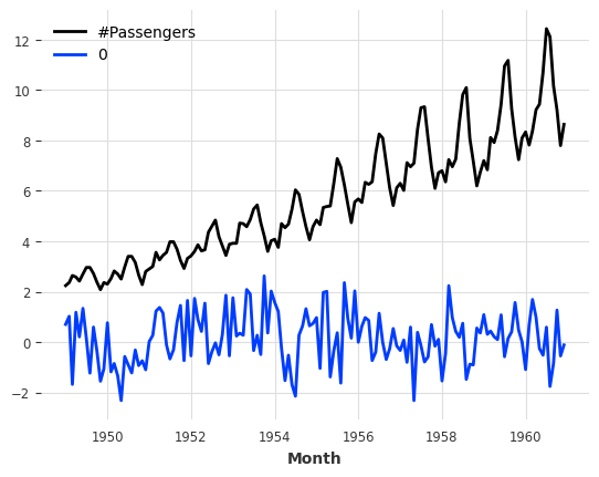
(series / 2 + 20 * series_noise - 10).plot();
Stacking
Concatenating a new dimension to produce a new single multivariate series.
[9]:
(series / 50).stack(series_noise).plot();
Mapping:
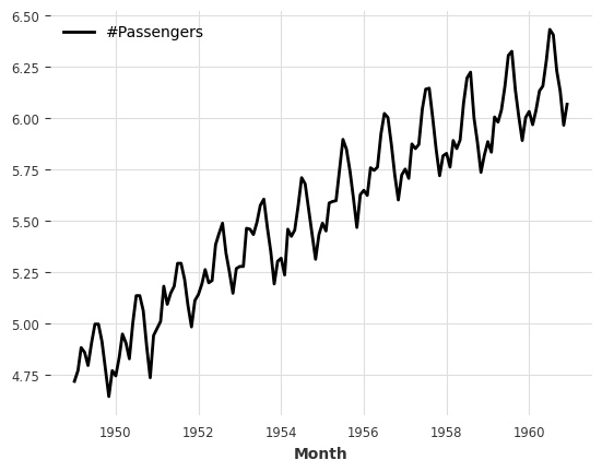
[10]:
series.map(np.log).plot();
Mapping on both timestamps and values:
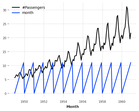
[11]:
series.map(lambda ts, x: x / ts.days_in_month.values.reshape(-1, 1, 1)).plot();
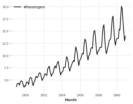
Adding some datetime attribute as an extra dimension (yielding a multivariate series):
[12]:
(series / 20).add_datetime_attribute("month").plot();
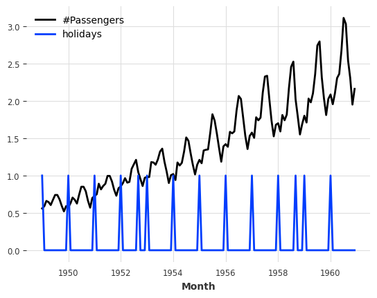
Adding some binary holidays component:
[13]:
(series / 200).add_holidays("US").plot();
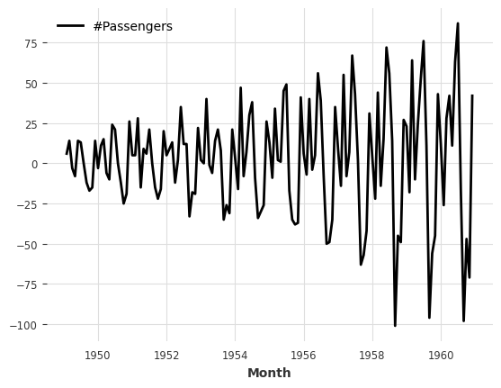
Differencing:
[14]:
series.diff().plot();
Filling missing values (using a ``utils`` function).
Missing values are represented by np.nan.
[15]:
from darts.utils.missing_values import fill_missing_values

values = np.arange(50, step=0.5)
values[10:30] = np.nan
values[60:95] = np.nan
series_ = TimeSeries.from_values(values)

(series_ - 10).plot(label="with missing values (shifted below)")
fill_missing_values(series_).plot(label="without missing values");
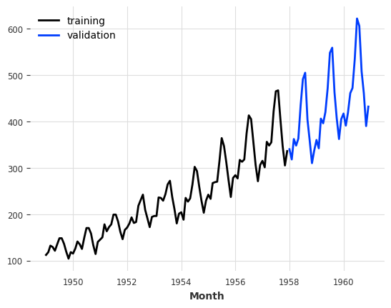
Creating a training and validation series#
For what follows, we will split our TimeSeries into a training and a validation series. Note: in general, it is also a good practice to keep a test series aside and never touch it until the end of the process. Here, we just build a training and a validation series for simplicity.
The training series will be a TimeSeries containing values until January 1958 (excluded), and the validation series a TimeSeries containing the rest:
[16]:
train, val = series.split_before(pd.Timestamp("19580101"))
train.plot(label="training")
val.plot(label="validation");
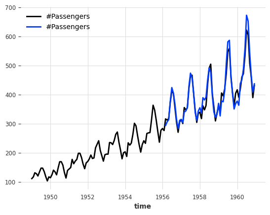
Training forecasting models and making predictions#
Playing with toy models#
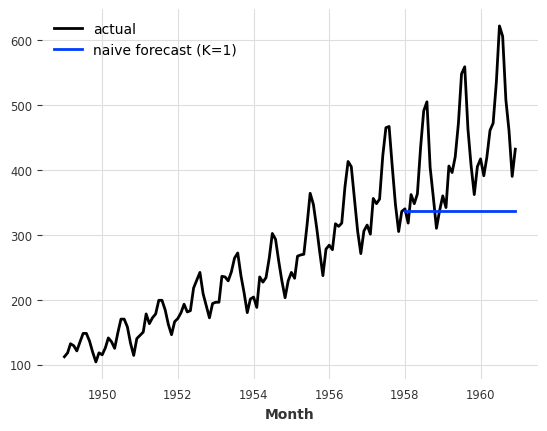
There is a collection of “naive” baseline models in Darts, which can be very useful to get an idea of the bare minimum accuracy that one could expect. For example, the NaiveSeasonal(K) model always “repeats” the value that occured K time steps ago.
In its most naive form, when K=1, this model simply always repeats the last value of the training series:
[17]:
from darts.models import NaiveSeasonal

naive_model = NaiveSeasonal(K=1)
naive_model.fit(train)
naive_forecast = naive_model.predict(36)

series.plot(label="actual")
naive_forecast.plot(label="naive forecast (K=1)");
It’s very easy to fit models and produce predictions on TimeSeries. All the models have a fit() and a predict() function. This is similar to Scikit-learn, except that it is specific to time series. The fit() function takes as argument the training time series on which to fit the model, and the predict() function takes as argument the number of time steps (after the end of the training series) over which to forecast.
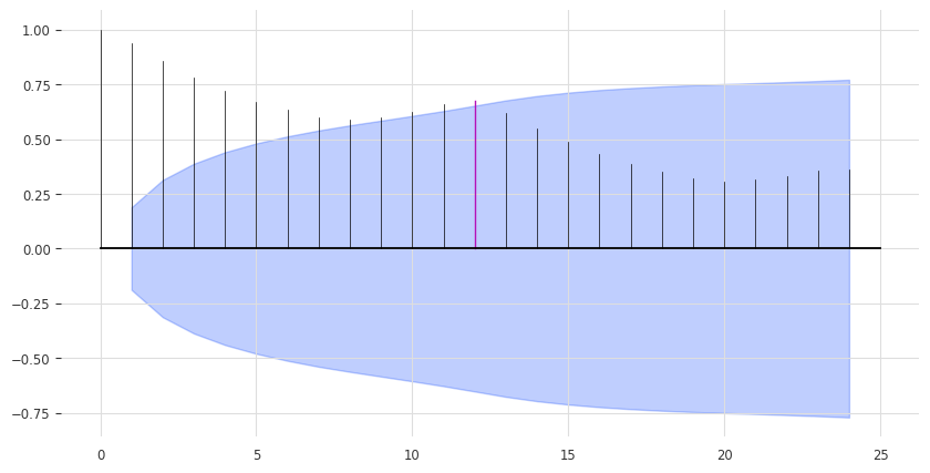
Inspect Seasonality#
Our model above is perhaps a bit too naive. We can already improve by exploiting the seasonality in the data. It seems quite obvious that the data has a yearly seasonality, which we can confirm by looking at the auto-correlation function (ACF), and highlighting the lag m=12:
[18]:
from darts.utils.statistics import check_seasonality, plot_acf

plot_acf(train, m=12, alpha=0.05, max_lag=24)

The ACF presents a spike at x = 12, which suggests a yearly seasonality trend (highlighted in red). The blue zone determines the significance of the statistics for a confidence level of \(\alpha = 5\%\). We can also run a statistical check of seasonality for each candidate period m:
[19]:
for m in range(2, 25):
    is_seasonal, period = check_seasonality(train, m=m, alpha=0.05)
    if is_seasonal:
        print(f"There is seasonality of order {period}.")
There is seasonality of order 12.
A less naive model#
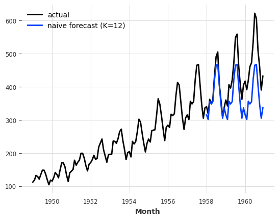
Let’s try the NaiveSeasonal model again with a seasonality of 12:
[20]:
seasonal_model = NaiveSeasonal(K=12)
seasonal_model.fit(train)
seasonal_forecast = seasonal_model.predict(36)

series.plot(label="actual")
seasonal_forecast.plot(label="naive forecast (K=12)");
This is better, but we are still missing the trend. Fortunately, there is also another naive baseline model capturing the trend, which is called NaiveDrift. This model simply produces linear predictions, with a slope that is determined by the first and last values of the training set:
[21]:
from darts.models import NaiveDrift

drift_model = NaiveDrift()
drift_model.fit(train)
drift_forecast = drift_model.predict(36)

combined_forecast = drift_forecast + seasonal_forecast - train.last_value()

series.plot()
combined_forecast.plot(label="combined")
drift_forecast.plot(label="drift");
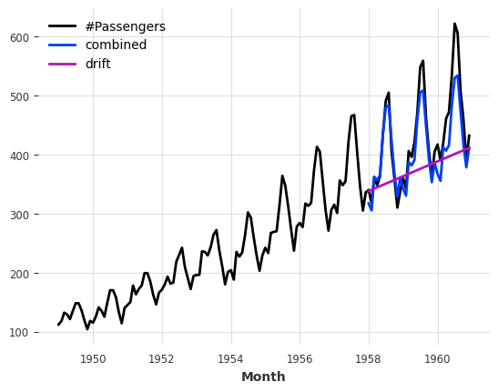
What happened there? We simply fit a naive drift model, and add its forecast to the seasonal forecast we had previously. We also subtract the last value of the training set from the result, so that the resulting combined forecast starts off with the right offset.
Computing error metrics#
This looks already like a fairly decent forecast, and we did not use any non-naive model yet. In fact - any model should be able to beat this.
So what’s the error we will have to beat? We will use the Mean Absolute Percentage Error (MAPE) (note that in practice there are often good reasons not to use the MAPE - we use it here as it is quite convenient and scale independent). In Darts it is a simple function call:
[22]:
from darts.metrics import mape

print(
    f"Mean absolute percentage error for the combined naive drift + seasonal: {mape(series, combined_forecast):.2f}%."
)
Mean absolute percentage error for the combined naive drift + seasonal: 5.66%.
darts.metrics contains many more metrics to compare time series. The metrics will compare only common slices of series when the two series are not aligned, and parallelize computation over a large number of series pairs - but let’s not get ahead of ourselves.
Quickly try out several models#
Darts is built to make it easy to train and validate several models in a unified way. Let’s train a few more and compute their respective MAPE on the validation set:
[23]:
from darts.models import AutoARIMA, ExponentialSmoothing, Theta


def eval_model(model):
    model.fit(train)
    forecast = model.predict(len(val))
    print(f"model {model} obtains MAPE: {mape(val, forecast):.2f}%")


eval_model(ExponentialSmoothing())
eval_model(AutoARIMA())
eval_model(Theta())
model ExponentialSmoothing() obtains MAPE: 5.11%
model AutoARIMA() obtains MAPE: 12.70%
model Theta() obtains MAPE: 8.15%
Here, we only created these models with their default parameters. We can probably do better if we fine-tune to our problem. Let’s try with the Theta method.
Searching for hyper-parameters with the Theta method#
The model Theta contains an implementation of Assimakopoulos and Nikolopoulos’ Theta method. This method has had some success, particularly in the M3-competition.
Though the value of the Theta parameter is often set to 0 in applications, our implementation supports a variable value for parameter tuning purposes. Let’s try to find a good value for Theta:
[24]:
# Search for the best theta parameter, by trying 50 different values
thetas = 2 - np.linspace(-10, 10, 50)

best_mape = float("inf")
best_theta = 0

for theta in thetas:
    model = Theta(theta)
    model.fit(train)
    pred_theta = model.predict(len(val))
    res = mape(val, pred_theta)

    if res < best_mape:
        best_mape = res
        best_theta = theta
[25]:
best_theta_model = Theta(best_theta)
best_theta_model.fit(train)
pred_best_theta = best_theta_model.predict(len(val))

print(f"Lowest MAPE is: {mape(val, pred_best_theta):.2f}, with theta = {best_theta}.")
Lowest MAPE is: 4.40, with theta = -3.5102040816326543.
[26]:
train.plot(label="train")
val.plot(label="true")
pred_best_theta.plot(label="prediction");
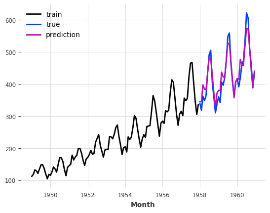
We can observe that the model with best_theta is so far the best we have, in terms of MAPE.
Backtesting: simulate historical forecasting#
So at this point we have a model that performs well on our validation set, and that’s good. But, how can we know the performance we would have obtained if we had been using this model historically?
Backtesting simulates predictions that would have been obtained historically with a given model. It can take a while to produce, since the model is (by default) re-trained every time the simulated prediction time advances.
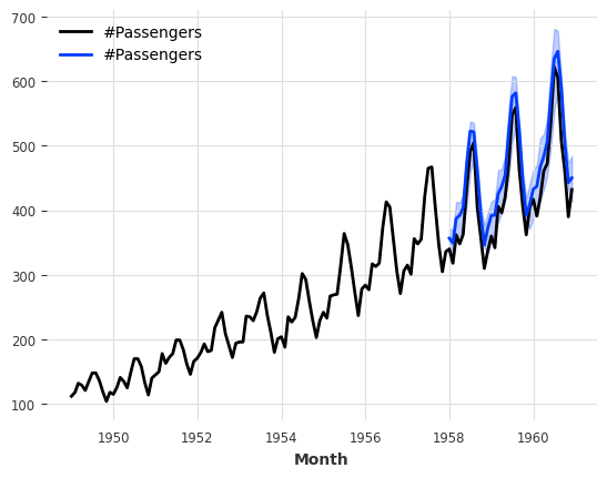
Such simulated forecasts are always defined with respect to a forecast horizon, which is the number of time steps that separate the prediction time from the forecast time. In the example below, we simulate forecasts done for 3 months into the future (compared to prediction time). The result of calling historical_forecasts() is (by default) a TimeSeries which contains only the last predicted value of each of those 3-months ahead forecasts:
[27]:
hfc_params = {
"series": series,
"start": pd.Timestamp(
"1956-01-01"
), # can also be a float for the fraction of the series to start at
"forecast_horizon": 3,
"verbose": True,
}
historical_fcast_theta = best_theta_model.historical_forecasts(
last_points_only=True, **hfc_params
)
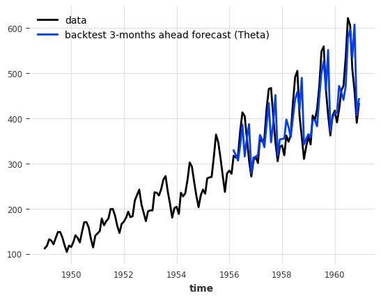
series.plot(label="data")
historical_fcast_theta.plot(label="backtest 3-months ahead forecast (Theta)")
print(f"MAPE = {mape(series, historical_fcast_theta):.2f}%")
MAPE = 7.99%
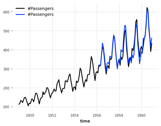
We can also retrieve all predicted values from each historical forecast, by setting last_points_only=False. With the stride parameter we define how many steps to move between two consecutative forecasts. We set it to 3 months, so that we can then concatenate the forecasts into a single TimeSeries.
[28]:
historical_fcast_theta_all = best_theta_model.historical_forecasts(
    last_points_only=False, stride=3, **hfc_params
)

series.plot(label="data")
for idx, hfc in enumerate(historical_fcast_theta_all):
    hfc.plot(label=f"forecast {idx}")

from darts import concatenate

historical_fcast_theta_all = concatenate(historical_fcast_theta_all, axis=0)
print(f"MAPE = {mape(series, historical_fcast_theta_all):.2f}%")
MAPE = 5.61%
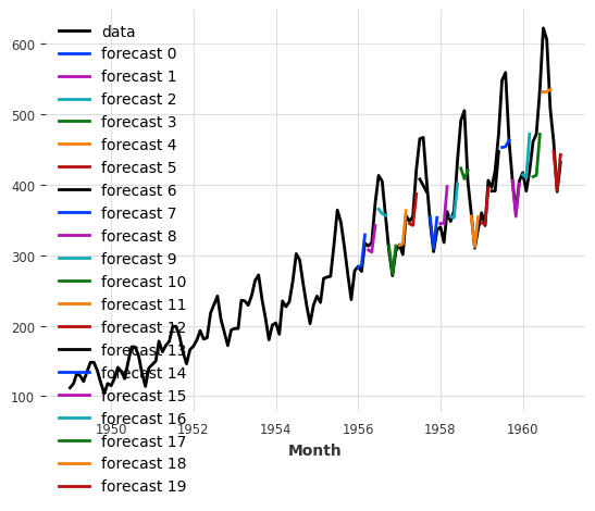
So it seems that our best model on validation set is not doing so great anymore when we backtest it (did I hear overfitting :D)
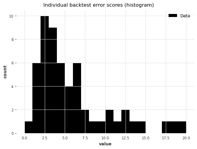
To have a closer look at the errors, we can also use the backtest() method to obtain all the raw errors (say, MAPE errors) that would have been obtained by our model:
[29]:
best_theta_model = Theta(best_theta)

raw_errors = best_theta_model.backtest(
    metric=mape, reduction=None, last_points_only=False, stride=1, **hfc_params
)

from darts.utils.statistics import plot_hist

plot_hist(
    raw_errors,
    bins=np.arange(0, max(raw_errors), 1),
    title="Individual backtest error scores (histogram)",
);
Finally, using backtest() we can also get a simpler view of the average error over the historical forecasts:
[30]:
average_error = best_theta_model.backtest(
    metric=mape,
    reduction=np.mean,  # this is actually the default
    **hfc_params,
)

print(f"Average error (MAPE) over all historical forecasts: {average_error:.2f}")
Average error (MAPE) over all historical forecasts: 6.30
We could also for instance have specified the argument reduction=np.median to get the median MAPE instead.
Above, backtest() re-computed the historical forecasts every time we called it. We can also use some pre-computed forecasts to get the results much faster!
[31]:
hfc_precomputed = best_theta_model.historical_forecasts(
    last_points_only=False, stride=1, **hfc_params
)
new_error = best_theta_model.backtest(
    historical_forecasts=hfc_precomputed, last_points_only=False, stride=1, **hfc_params
)

print(f"Average error (MAPE) over all historical forecasts: {new_error:.2f}")
Average error (MAPE) over all historical forecasts: 6.30
Looking at residuals#
Let’s look at the fitted value residuals of our current Theta model, i.e. the difference between the 1-step forecasts at every point in time obtained by fitting the model on all previous points, and the actual observed values:
[32]:
from darts.utils.statistics import plot_residuals_analysis

plot_residuals_analysis(best_theta_model.residuals(series))
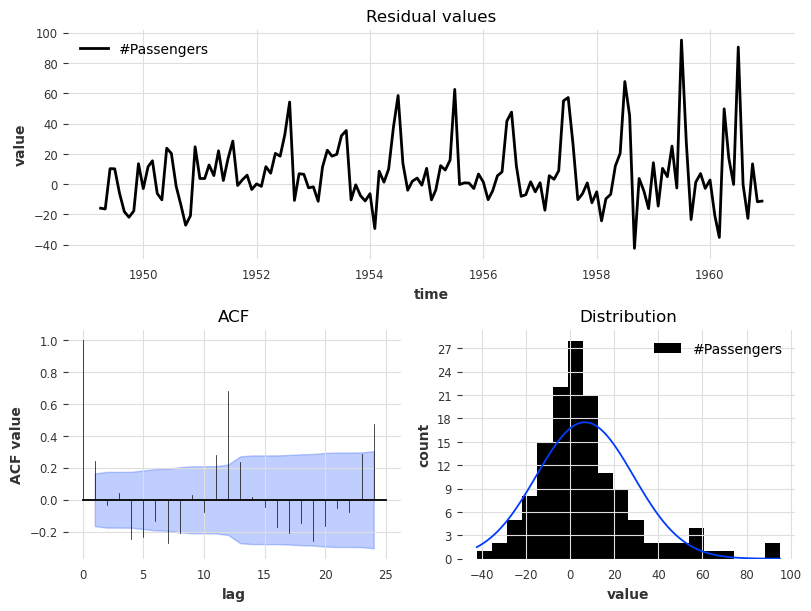
We can see that the distribution is not centered at 0, which means that our Theta model is biased. We can also make out a large ACF value at lag equal to 12, which indicates that the residuals contain information that was not used by the model.
Our residuals method is actually much more powerful! It can be used to compute any per-time step metric from Darts (see a list here) even for multi-step forecasts. It also supports pre-computed historical forecasts similar to backtest.
Now let’s check the distribution of absolute errors we get for each step in the 3 months forecasts.
[33]:
from darts.metrics import ae

residuals = best_theta_model.residuals(
    historical_forecasts=hfc_precomputed,
    metric=ae,  # the absolute error per time step
    last_points_only=False,
    values_only=True,  # return a list of numpy arrays
    **hfc_params,
)
residuals = np.concatenate(residuals, axis=1)[:, :, 0]

fig, ax = plt.subplots()
for forecast_step in range(len(residuals)):
    ax.hist(residuals[forecast_step], label=f"step {forecast_step}", alpha=0.5)
ax.legend()
ax.set_title("Absolute errors per forecast step");
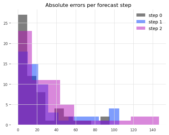
We can clearly see that the errors increase the further ahead into the future we predict.
A better model#
Could we maybe do better with a simple ExponentialSmoothing model?
[34]:
model_es = ExponentialSmoothing(seasonal_periods=12)
historical_fcast_es = model_es.historical_forecasts(**hfc_params)

series.plot(label="data")
historical_fcast_es.plot(label="backtest 3-months ahead forecast (Exp. Smoothing)")
print(f"MAPE = {mape(historical_fcast_es, series):.2f}%")
MAPE = 4.42%
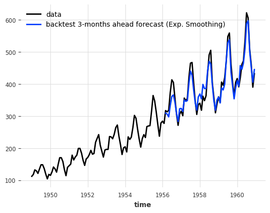
This is much better! We get a mean absolute percentage error of about 4-5% when backtesting with a 3-months forecast horizon in this case.
[35]:
plot_residuals_analysis(model_es.residuals(series, verbose=True))
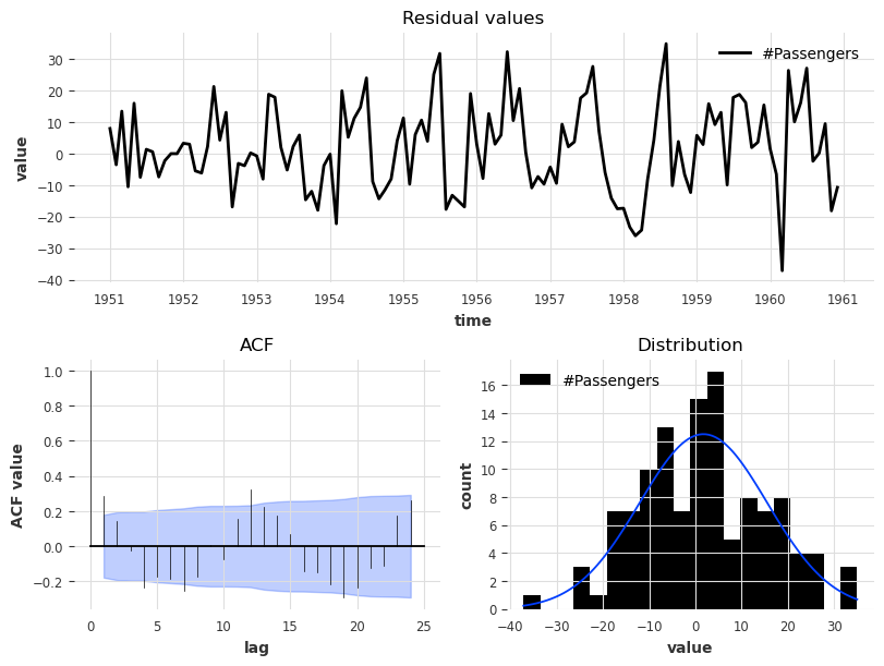
The residual analysis also reflects an improved performance in that we now have a distribution of the residuals centred at value 0, and the ACF values, although not insignificant, have lower magnitudes.
Machine learning and global models#
Darts has a rich support for machine learning and deep learning forecasting models; for instance:
SKLearnModel can wrap around any sklearn-compatible regression model to produce forecasts (it has its own section below).
RNNModel is a flexible RNN implementation, which can be used like DeepAR.
NBEATSModel implements the N-BEATS model.
TFTModel implements the Temporal Fusion Transformer model.
TCNModel implements temporal convolutional networks.
…
In addition to supporting the same basic fit()/predict() interface as the other models, these models are also global models, as they support being trained on multiple time series (sometimes referred to as meta learning).
This is a key point of using ML-based models for forecasting: more often than not, ML models (especially deep learning models) need to be trained on large amounts of data, which often means a large amount of separate yet related time series.
In Darts, the basic way to specify multiple TimeSeries is using a Sequence of TimeSeries (for example, a simple list of TimeSeries).
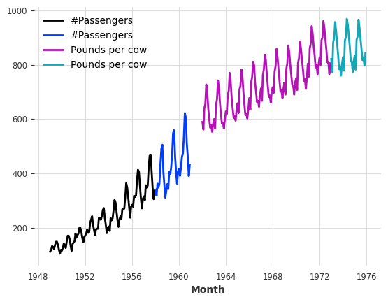
A toy example with two series#
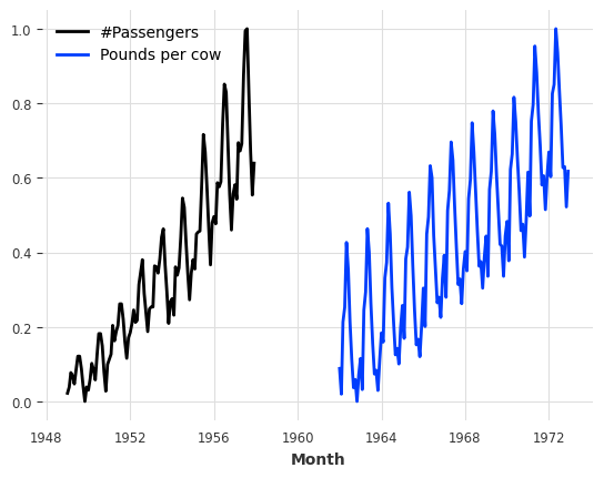
These models can be trained on thousands of series. Here, for the sake of illustration, we will load two distinct series - the air traffic passenger count and another series with the number of pounds of milk produced per cow monthly. We also cast our series to np.float32 as that will slightly speedup the training:
[36]:
from darts.datasets import AirPassengersDataset, MonthlyMilkDataset

series_air = AirPassengersDataset().load().astype(np.float32)
series_milk = MonthlyMilkDataset().load().astype(np.float32)

# set aside last 36 months of each series as validation set:
train_air, val_air = series_air[:-36], series_air[-36:]
train_milk, val_milk = series_milk[:-36], series_milk[-36:]

train_air.plot()
val_air.plot()
train_milk.plot()
val_milk.plot();
First, let’s scale these two series between 0 and 1, as that will benefit most ML models. We will use a Scaler for this:
[37]:
from darts.dataprocessing.transformers import Scaler

scaler = Scaler()
train_air_scaled, train_milk_scaled = scaler.fit_transform([train_air, train_milk])

train_air_scaled.plot()
train_milk_scaled.plot();
Note how we can scale several series in one go. We can also parallelize this sort of operations over multiple processors by specifying n_jobs.
Using deep learning: example with N-BEATS#
Note: You can find a detailed user guide for our Neural Network Models (TorchForecastingModels) here.
Next, we will build an N-BEATS model. This model can be tuned with many hyper-parameters (such as number of stacks, layers, etc). Here, for simplicity, we will use it with default hyper-parameters. The only two hyper-parameters that we have to provide are:
input_chunk_length: this is the “lookback window” of the model - i.e., how many time steps of history the neural network takes as input to produce its output in a forward pass.output_chunk_length: this is the “forward window” of the model - i.e., how many time steps of future values the neural network outputs in a forward pass.
The random_state parameter is just here to get reproducible results.
Most neural networks in Darts require these two parameters. Here, we will use multiples of the seasonality. We are now ready to fit our model on our two series (by giving a list containing the two series to fit()):
[38]:
from darts.models import NBEATSModel

model = NBEATSModel(input_chunk_length=24, output_chunk_length=12, random_state=42)

model.fit([train_air_scaled, train_milk_scaled], epochs=50, verbose=True);
GPU available: True (mps), used: True
TPU available: False, using: 0 TPU cores
HPU available: False, using: 0 HPUs

  | Name            | Type             | Params | Mode
-------------------------------------------------------------
0 | criterion       | MSELoss          | 0      | train
1 | train_criterion | MSELoss          | 0      | train
2 | val_criterion   | MSELoss          | 0      | train
3 | train_metrics   | MetricCollection | 0      | train
4 | val_metrics     | MetricCollection | 0      | train
5 | stacks          | ModuleList       | 6.2 M  | train
-------------------------------------------------------------
6.2 M     Trainable params
1.4 K     Non-trainable params
6.2 M     Total params
24.787    Total estimated model params size (MB)
396       Modules in train mode
0         Modules in eval mode
`Trainer.fit` stopped: `max_epochs=50` reached.
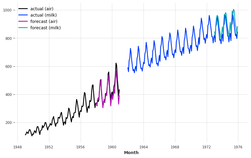
Let’s now get some forecasts 36 months ahead, for our two series. We can just use the series argument of the predict() function to tell the model which series to forecast. Importantly, the output_chunk_length does not directly constrain the forecast horizon n of predict(). Here, we trained the model with output_chunk_length=12 and produce forecasts for n=36 months ahead; this is simply done in an auto-regressive way behind the scenes (where the network recursively
consumes its previous outputs).
[39]:
pred_air, pred_milk = model.predict(series=[train_air_scaled, train_milk_scaled], n=36)

# scale back:
pred_air, pred_milk = scaler.inverse_transform([pred_air, pred_milk])

plt.figure(figsize=(10, 6))
series_air.plot(label="actual (air)")
series_milk.plot(label="actual (milk)")
pred_air.plot(label="forecast (air)")
pred_milk.plot(label="forecast (milk)");
GPU available: True (mps), used: True
TPU available: False, using: 0 TPU cores
HPU available: False, using: 0 HPUs
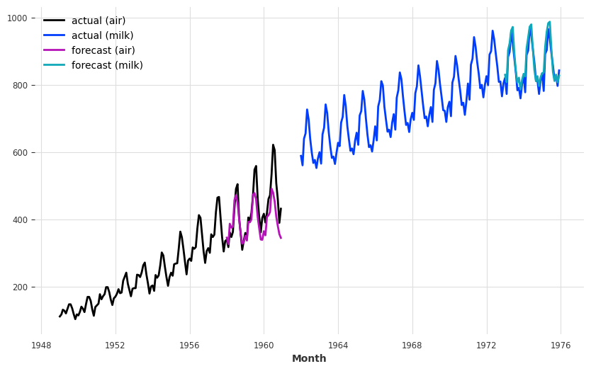
Our forecasts are actually not so terrible, considering that we use one model with default hyper-parameters to capture both air passengers and milk production!
The model seems quite OK at capturing the yearly seasonality, but misses the trend for the air series. In the next section, we will try to solve this issue using external data (covariates).
Covariates: using external data#
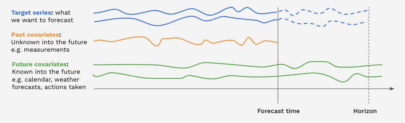
In addition to the target series (the series we are interested to forecast), many models in Darts also accept covariates series in input. Covariates are series that we do not want to forecast, but which can provide helpful additional information to the models. Both the targets and covariates can be multivariate or univariate.
There are two kinds of covariate time series in Darts:
past_covariatesare series not necessarily known ahead of the forecast time. They can for instance represent things that have to be measured and are not known upfront. Models do not use future values ofpast_covariateswhen making forecasts (only for global models when predicting withn > output_chunk_lengthdue to auto-regression). For more info on past/future covariates, check out this user guide.future_covariatesare series which are known in advance, up to the forecast horizon. They can represent things such as calendar information, holidays, weather forecasts, etc. Models that acceptfuture_covariateswill look at the future values (up to the forecast horizon) when making forecasts.static_covariatesare characteristics of the target series which do not change over time. They are embedded directly into the target series. They can represent things such as the category of product, country information, etc. For more info on static covariates, check out this user guide.
Each covariate can potentially be multivariate. If you have several covariate series (such as month and year values), you should stack() or concatenate() them to obtain a multivariate series.
The covariates you provide can be longer than necessary. Darts’s model will automatically handle the extraction of relevant time frames for you! You will receive an error if your covariates do not have a sufficient time span, though.
Not all models support every covariate type. You can find a model list here stating which types they support.
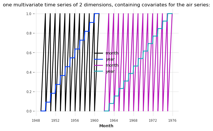
Let’s now build some external covariates containing both monthly and yearly values for our air and milk series. In the cell below, we use the darts.utils.timeseries_generation.datetime_attribute_timeseries() function to generate series containing the month and year values, and we concatenate() these series along the "component" axis (same as axis=1) in order to obtain one covariate series with two components (month and year), per target series. For simplicity, we directly scale
the month and year values to have them between 0 and 1:
[40]:
from darts import concatenate
from darts.utils.timeseries_generation import datetime_attribute_timeseries as dt_attr

air_covs = concatenate(
    [
        dt_attr(series_air, "month", dtype=np.float32),
        dt_attr(series_air, "year", dtype=np.float32),
    ],
    axis="component",
)

milk_covs = concatenate(
    [
        dt_attr(series_milk, "month", dtype=np.float32),
        dt_attr(series_milk, "year", dtype=np.float32),
    ],
    axis="component",
)

air_covs_scaled, milk_covs_scaled = Scaler().fit_transform([air_covs, milk_covs])
air_covs_scaled.plot()
milk_covs_scaled.plot()
plt.title(
    "one multivariate time series of 2 dimensions, containing covariates for the air series:"
);
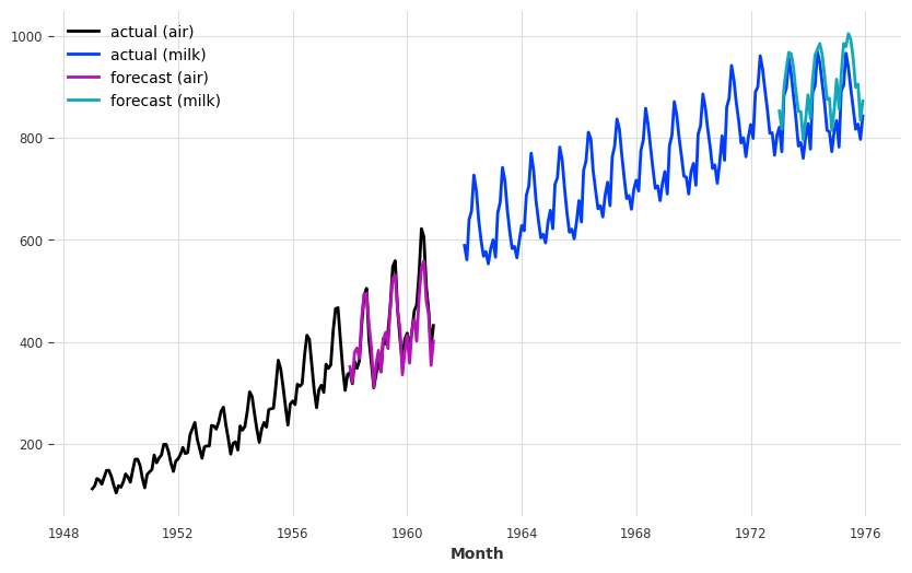
NBEATSModel supports only past_covariates. Therefore, even though our covariates represent calendar information and are known in advance, we will use them as past_covariates with N-BEATS. To train, all we have to do is give them as past_covariates to the fit() function, in the same order as the targets:
[41]:
model = NBEATSModel(input_chunk_length=24, output_chunk_length=12, random_state=42)

model.fit(
    [train_air_scaled, train_milk_scaled],
    past_covariates=[air_covs_scaled, milk_covs_scaled],
    epochs=50,
    verbose=True,
);
GPU available: True (mps), used: True
TPU available: False, using: 0 TPU cores
HPU available: False, using: 0 HPUs

  | Name            | Type             | Params | Mode
-------------------------------------------------------------
0 | criterion       | MSELoss          | 0      | train
1 | train_criterion | MSELoss          | 0      | train
2 | val_criterion   | MSELoss          | 0      | train
3 | train_metrics   | MetricCollection | 0      | train
4 | val_metrics     | MetricCollection | 0      | train
5 | stacks          | ModuleList       | 6.6 M  | train
-------------------------------------------------------------
6.6 M     Trainable params
1.7 K     Non-trainable params
6.6 M     Total params
26.314    Total estimated model params size (MB)
396       Modules in train mode
0         Modules in eval mode
`Trainer.fit` stopped: `max_epochs=50` reached.
Then to produce forecasts, we again have to provide our covariates as past_covariates to the predict() function.
[42]:
preds = model.predict(
    series=[train_air_scaled, train_milk_scaled],
    past_covariates=[air_covs_scaled, milk_covs_scaled],
    n=36,
)

# scale back:
pred_air, pred_milk = scaler.inverse_transform(preds)

plt.figure(figsize=(10, 6))
series_air.plot(label="actual (air)")
series_milk.plot(label="actual (milk)")
pred_air.plot(label="forecast (air)")
pred_milk.plot(label="forecast (milk)");
`predict()` was called with `n > output_chunk_length`: using auto-regression to forecast the values after `output_chunk_length` points. The model will access `(n - output_chunk_length)` future values of your `past_covariates` (relative to the first predicted time step). To hide this warning, set `show_warnings=False`.
GPU available: True (mps), used: True
TPU available: False, using: 0 TPU cores
HPU available: False, using: 0 HPUs
It seems that now the model captures the trend of the air series better (which also perturbs a bit the forecasts of the milk series).
The model warning is pretty important. It tells us that future values of our past_covariates were used for prediction because we picked a hoizon n > output_chunk_length which activates auto-regression. The model will then cosume it’s own predictions as input for the next prediction. Since the prediction point moves ahead, the model requires new values from the past covariates. These will however only be extracted from the past relative to the prediciton point (never from the forecast
horizon itself)!
In our case it’s fine to do this since we only use calendar information that we know in advance. If instead we used some features that we only know in the past, then we should only forecast with n <= output_chunk_length.
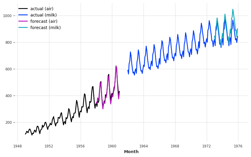
Encoders: using covariates for free#
Using covariates related to the calendar or time axis (such as months and years as in our example above) is so frequent that all of Darts’ models with covariates support have a built-in functionality to generate them out of the box.
To easily integrate such covariates to your model, you can simply specify the add_encoders parameter at model creation. This parameter has to be a dictionary containing informations about what should be encoded as extra covariates. Here is an example of what such a dictionary could look like, for a model supporting both past and future covariates:
[43]:
def extract_year(idx):
    """Extract the year each time index entry and normalized it."""
    return (idx.year - 1950) / 50


encoders = {
    "cyclic": {"future": ["month"]},
    "datetime_attribute": {"future": ["hour", "dayofweek"]},
    "position": {"past": ["absolute"], "future": ["relative"]},
    "custom": {"past": [extract_year]},
    "transformer": Scaler(),
}
In the above dictionary, the following things are specified:
The month should be used as a future covariate, with a cyclic (sin/cos) encoding.
The hour and day-of-the-week should be used as future covariates.
The absolute position (time step in the series) should be used as past covariates.
The relative position (w.r.t the forecasting time) should be used as future covariates.
An additional custom function of the year should be used as past covariates.
All the above covariates should be scaled using a
Scaler, which will be fit upon calling the modelfit()function and used afterwards to transform the covariates.
We refer to the API doc for more informations about how to use encoders. Note that lambda functions cannot be used as they are not pickable.
To replicate our example with month and year used as past covariates with N-BEATS, we can use some encoders as follows:
[44]:
encoders = {"datetime_attribute": {"past": ["month", "year"]}, "transformer": Scaler()}
Now, the whole training of the N-BEATS model with these covariates looks as follows:
[45]:
model = NBEATSModel(
    input_chunk_length=24,
    output_chunk_length=12,
    add_encoders=encoders,
    random_state=42,
)

model.fit([train_air_scaled, train_milk_scaled], epochs=50, verbose=True);
GPU available: True (mps), used: True
TPU available: False, using: 0 TPU cores
HPU available: False, using: 0 HPUs

  | Name            | Type             | Params | Mode
-------------------------------------------------------------
0 | criterion       | MSELoss          | 0      | train
1 | train_criterion | MSELoss          | 0      | train
2 | val_criterion   | MSELoss          | 0      | train
3 | train_metrics   | MetricCollection | 0      | train
4 | val_metrics     | MetricCollection | 0      | train
5 | stacks          | ModuleList       | 6.6 M  | train
-------------------------------------------------------------
6.6 M     Trainable params
1.7 K     Non-trainable params
6.6 M     Total params
26.314    Total estimated model params size (MB)
396       Modules in train mode
0         Modules in eval mode
`Trainer.fit` stopped: `max_epochs=50` reached.
And get some forecasts for the air passengers series:
[46]:
preds = model.predict(
    series=[train_air_scaled, train_milk_scaled], n=36, show_warnings=False
)

# scale back:
pred_air, pred_milk = scaler.inverse_transform(preds)

plt.figure(figsize=(10, 6))
series_air.plot(label="actual (air)")
series_milk.plot(label="actual (milk)")
pred_air.plot(label="forecast (air)")
pred_milk.plot(label="forecast (milk)");
GPU available: True (mps), used: True
TPU available: False, using: 0 TPU cores
HPU available: False, using: 0 HPUs
Regression forecasting models#
Note: You can find a detailed example notebook for our SKLearnModel here.
SKLearnModel are forecasting models which wrap around sklearn-compatible regression models. The inner regression model is used to predict future values of the target series, as a function of certain lags of the target, past and future covariates. Behind the scenes, the time series are tabularized in order to build a training dataset in the right format.
By default, the SKLearnModel will do a linear regression. It is very easy to use any desired sklearn-compatible regression model by specifying the model parameter, but for convenience Darts also provides a couple of ready-made models out of the box:
LinearRegressionModel wraps around
sklearn.linear_model.LinearRegression(accepting the same kwargs).RandomForestModel wraps around
sklearn.ensemble.RandomForestRegressor.LightGBMModel wraps around
lightbm.XGBModel wraps around
xgboost.CatBoostModel wraps around
catboost.
For example, this is what fitting a Bayesian ridge regression to our toy two-series problem looks like:
[ ]:
from sklearn.linear_model import BayesianRidge

from darts.models import SKLearnModel

model = SKLearnModel(lags=72, lags_future_covariates=[-6, 0], model=BayesianRidge())

model.fit(
    [train_air_scaled, train_milk_scaled],
    future_covariates=[air_covs_scaled, milk_covs_scaled],
);
Several things happened above:
lags=72is telling theSKLearnModelto look at the past 72 lags / months of the target.In addition,
lags_future_covariates=[-6, 0]means that the model will also look at lags of thefuture_covariateswe provide. Here we specify the exact lags we want the models to take into account; the “-6th” and the “0th” lag. The “0th” lag means the “current” lag (i.e., at the time step being forecasted); obviously, knowning this lag requires knowing the data in advance (hence the fact we are usingfuture_covariates). Similarly,-6means we also look at the value of the covariates 6 months before the forecasted time step (which also requires to know the covariates in advance if we are forecasting at a horizon more than 6 steps ahead).model=BayesianRidge()provides the actual inner regression model.
Now let’s get some forecasts:
[48]:
preds = model.predict(
    series=[train_air_scaled, train_milk_scaled],
    future_covariates=[air_covs_scaled, milk_covs_scaled],
    n=36,
)

# scale back:
pred_air, pred_milk = scaler.inverse_transform(preds)

plt.figure(figsize=(10, 6))
series_air.plot(label="actual (air)")
series_milk.plot(label="actual (milk)")
pred_air.plot(label="forecast (air)")
pred_milk.plot(label="forecast (milk)");
Note how we obtained the forecasts for the two time series at once above. Similarly, we can also get some metrics over sequences of series:
[49]:
mape([series_air, series_milk], [pred_air, pred_milk])
[49]:
[3.435389, 5.129032]
or the average metric over “all” series:
[50]:
mape([series_air, series_milk], [pred_air, pred_milk], series_reduction=np.mean)
[50]:
4.2822104
It seems that this model performs well on the Air traffic series, how does it do when we backtest it on this one series?
[ ]:
bayes_ridge_model = SKLearnModel(
    lags=72, lags_future_covariates=[0], model=BayesianRidge()
)

backtest = bayes_ridge_model.historical_forecasts(
    future_covariates=[air_covs_scaled, milk_covs_scaled],
    **hfc_params,
)

print(f"MAPE = {mape(series_air, backtest):.2f}%")
series_air.plot()
backtest.plot();
`enable_optimization=True` is ignored because `retrain` is not `False` or `0`. To hide this warning, set `show_warnings=False` or `enable_optimization=False`.
`enable_optimization=True` is ignored because `forecast_horizon > model.output_chunk_length`. To hide this warning, set `show_warnings=False` or `enable_optimization=False`.
MAPE = 3.76%
Our best model so far!
Applying scaler in backtesting#
To avoid data-leakage through the target and future covariate scaler, we will pass it to historical_forecasts so that the scaler is fitted and applied to both the target and the future covariates at each iteration.
[52]:
backtest_auto_scaling = bayes_ridge_model.historical_forecasts(
    future_covariates=air_covs,
    data_transformers={"series": Scaler(), "future_covariates": Scaler()},
    retrain=True,  # ensure that the scalers are fitted at each iterations
    **hfc_params,
)

print(f"MAPE = {mape(series_air, backtest_auto_scaling):.2f}%")
series_air.plot()
backtest_auto_scaling.plot();
`enable_optimization=True` is ignored because `retrain` is not `False` or `0`. To hide this warning, set `show_warnings=False` or `enable_optimization=False`.
`enable_optimization=True` is ignored because `forecast_horizon > model.output_chunk_length`. To hide this warning, set `show_warnings=False` or `enable_optimization=False`.
MAPE = 3.92%

The MAPE score is slightly worse, which is expected since information cannot leak from the future anymore but the backtesting conditions are more reliable.
Sample Weights#
All our global models (regression-, ensemble-, and neural network models) support sample weights for training. They are applied per observation, label (each step in output_chunk_length), and component. This can be very useful to:
weigh certain time frames more than others (e.g. decaying weights the further the points in the past, higher weights for times with more business value, …)
reduce / remove the effect of outliers or missing values on the model
Let’s just introduce some outliers to the air passengers series and see how a linear regression model with a 12 months lookback window (lags=12) performs on this data.
[53]:
# convert to pandas DataFrame and add some outliers
air_df = series_air.to_dataframe()
outlier_mask = (air_df.index.year >= 1950) & (air_df.index.year <= 1951)
air_df.loc[outlier_mask] = 600.0
air_outlier = TimeSeries.from_dataframe(air_df)

from darts.models import LinearRegressionModel

model_lin = LinearRegressionModel(lags=12, lags_future_covariates=[0])
hist_fc_kwargs = {
    "series": air_outlier,
    "future_covariates": air_covs_scaled,
    "start": 0.6,
    "forecast_horizon": 3,
    "verbose": True,
    "show_warnings": False,
}
backtest = model_lin.historical_forecasts(**hist_fc_kwargs)

print(f"MAPE = {mape(air_outlier, backtest):.2f}%")
air_outlier.plot(label="air series with outliers")
backtest.plot(label="non-weighted predictions");
MAPE = 26.40%
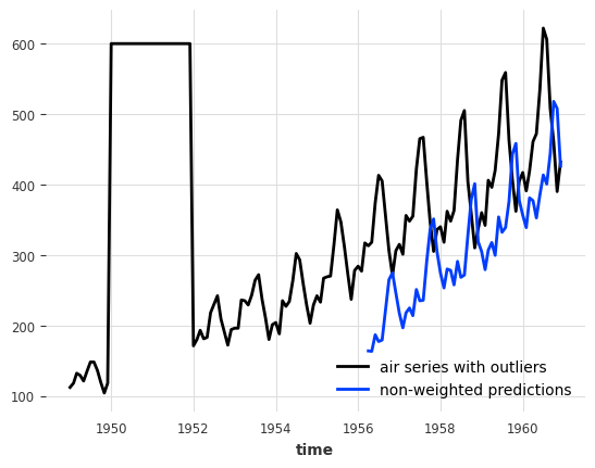
This doesn’t look very good. It would be great if we could ignore the outliers somehow. And this is where sample weights come in!
In Darts, sample weights are treated like covariates - they are defined as TimeSeries themselves. Thanks to that our models can automatically extract the relevant time frames for us!
Let’s create a weights series in which we set all outlier times to 0. and the remaining times to 1.. We also set the 12 months after the last outlier to 0., since these times fall into the lookback window of our model. Otherwise we would still have some outliers in the model input.
[54]:
weight_mask = (air_df.index.year >= 1950) & (air_df.index.year <= 1952)
sample_weight = np.ones((len(air_df), 1))
sample_weight[weight_mask, 0] = 0.0
sample_weight = air_outlier.with_values(sample_weight)

# and plot the results
air_outlier.plot(label="air series with outliers")
(sample_weight * 300).plot(label="sample weight * 300");
Now we can train the models with the sample weights using methods fit(), historical_forecasts, backtest(), …
[55]:
model_lin = LinearRegressionModel(lags=12, lags_future_covariates=[0])
backtest_weighted = model_lin.historical_forecasts(
    sample_weight=sample_weight, **hist_fc_kwargs
)

print(f"MAPE = {mape(series_air, backtest_weighted):.2f}%")
air_outlier.plot(label="air series with outliers")
backtest_weighted.plot(label="weighted predictions");
MAPE = 5.19%
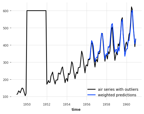
Wow, this looks great! We managed to completely remove the negative impact of the outliers on our model!
Note: our sample weights also support multi-horizon forecasts, multiple time series, multivariate series, and weights for evaluation sets (if the model support it)
Forecast Start Shifting#
We might also be interested in forecasts starting with an offset after the end of our target series. This can be useful for example:
In (Day-) Ahead Markets, where (each day) we need to make some biddings for a future point in time (next day) - we are not really interested in what happens between now and that future point in time. We can reduce model complexity by only focusing on times of interest.
When are covariates (or target series) are reported with a delay
All our global models support such predictions with an offset through model creation parameter output_chunk_shift - the number of steps to shift the first predicted step into the future.
With an output shift, the model cannot perform auto-regression anymore. So let’s create a linear model that directly predicts the next 12 months with an offset of 12 months.
[56]:
model_shifted = LinearRegressionModel(
    lags=12,
    lags_future_covariates=(0, 12),
    output_chunk_length=12,
    output_chunk_shift=12,
)

model_shifted.fit(series_air[:-24], future_covariates=air_covs)
preds = model_shifted.predict(n=12)

series_air[:-24].plot(label="train series")
series_air[-24:].plot(label="val_series")
preds.plot(label="shifted prediction");
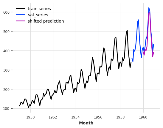
We see that the prediction starts 12 months after the end of the training series.
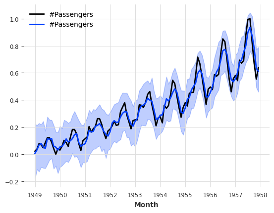
Probabilistic forecasts#
Most models in Darts support probabilistic forecasts (some local models and all regression-, ensemble- and neural network models). The full support list is available on the Darts README page.
With Local Models#
For local models (ARIMA, ExponentialSmoothing, …), we can simply specify a num_samples parameter when calling predict(). The returned TimeSeries will then contain num_samples Monte Carlo samples describing the distribution of the time series’ values. The advantage of relying on Monte Carlo samples (in contrast to, say, explicit confidence intervals) is that they can be used to describe any parametric or non-parametric joint distribution over components, and compute
arbitrary quantiles.
[57]:
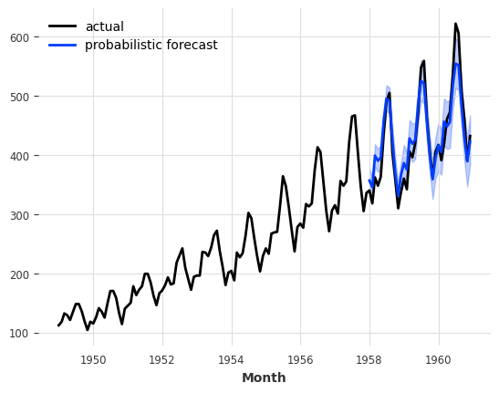
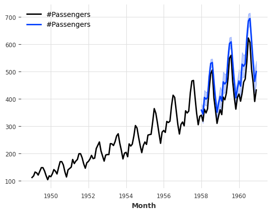
model_es = ExponentialSmoothing()
model_es.fit(train)
probabilistic_forecast = model_es.predict(len(val), num_samples=500)

series.plot(label="actual")
probabilistic_forecast.plot(label="probabilistic forecast")
plt.legend()
plt.show()

With Neural Network Models (TorchForecastingModel)#
With neural networks, we have to use a Likelihood object at model creation. The likelihoods specify which distribution the model will try to fit, along with potential prior values for the distributions’ parameters. The full list of available likelihoods is available in the docs.
Next to the distributions, we also support QuantileRegression as likelihood, which estimates future quantile values of the target series.
Using likelihoods is easy. For instance, here is what training an TCNModel to fit a Laplace likelihood looks like:
[58]:
from darts.models import TCNModel
from darts.utils.likelihood_models.torch import LaplaceLikelihood

model = TCNModel(
    input_chunk_length=24,
    output_chunk_length=12,
    random_state=42,
    likelihood=LaplaceLikelihood(),
    pl_trainer_kwargs={"accelerator": "cpu"},
)

model.fit(train_air_scaled, epochs=400, verbose=True);
GPU available: True (mps), used: False
TPU available: False, using: 0 TPU cores
HPU available: False, using: 0 HPUs
/Users/dennisbader/miniconda3/envs/darts/lib/python3.10/site-packages/pytorch_lightning/trainer/setup.py:177: GPU available but not used. You can set it by doing `Trainer(accelerator='gpu')`.

  | Name            | Type             | Params | Mode
-------------------------------------------------------------
0 | criterion       | MSELoss          | 0      | train
1 | train_criterion | MSELoss          | 0      | train
2 | val_criterion   | MSELoss          | 0      | train
3 | train_metrics   | MetricCollection | 0      | train
4 | val_metrics     | MetricCollection | 0      | train
5 | res_blocks      | ModuleList       | 166    | train
-------------------------------------------------------------
166       Trainable params
0         Non-trainable params
166       Total params
0.001     Total estimated model params size (MB)
23        Modules in train mode
0         Modules in eval mode
IOPub message rate exceeded.
The Jupyter server will temporarily stop sending output
to the client in order to avoid crashing it.
To change this limit, set the config variable
`--ServerApp.iopub_msg_rate_limit`.

Current values:
ServerApp.iopub_msg_rate_limit=1000.0 (msgs/sec)
ServerApp.rate_limit_window=3.0 (secs)
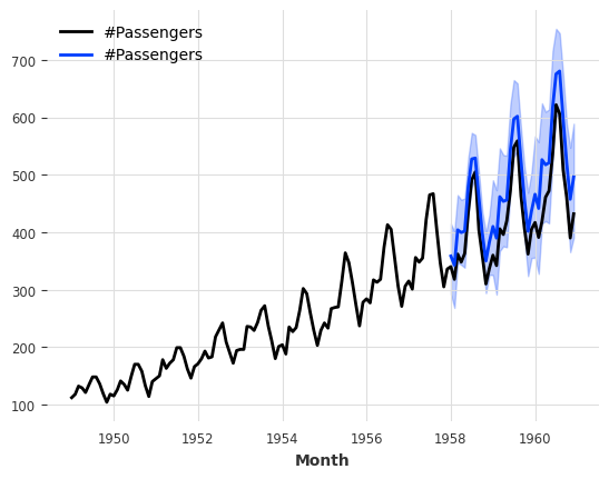
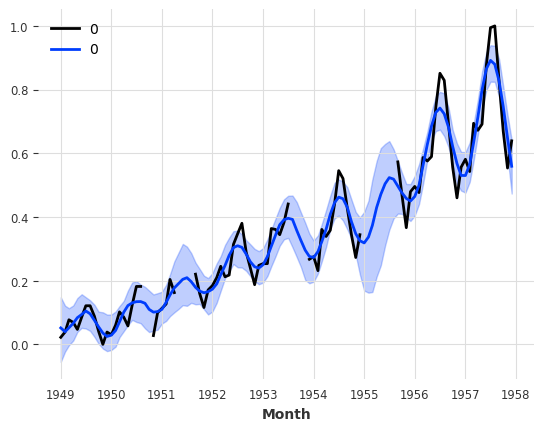
Probabilistic Sample Predictions#
Then to get probabilistic forecasts, we again only need to specify some num_samples >> 1. This will sample from predicted distribution.
[59]:
pred = model.predict(n=36, num_samples=500)

# scale back:
pred = scaler.inverse_transform(pred, series_idx=0)

series_air.plot()
pred.plot();
GPU available: True (mps), used: False
TPU available: False, using: 0 TPU cores
HPU available: False, using: 0 HPUs
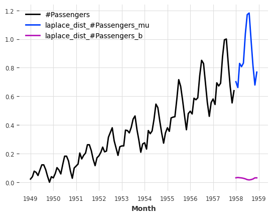
Direct Parameter Predicitons#
The great thing about our likelihoods is that instead of sampling from the distribution/quantiles, we can directly predict the distribution/quantile parameters. For this, we only have to set predict_likelihood_parameters=True.
Below we get the predicted location (mu) and scale (b) of the laplace distribution (in the scaled space between 0 and 1).
[60]:
pred = model.predict(n=12, predict_likelihood_parameters=True)

train_air_scaled.plot()
pred.plot(label="laplace_dist");
GPU available: True (mps), used: False
TPU available: False, using: 0 TPU cores
HPU available: False, using: 0 HPUs
/Users/dennisbader/miniconda3/envs/darts/lib/python3.10/site-packages/pytorch_lightning/trainer/setup.py:177: GPU available but not used. You can set it by doing `Trainer(accelerator='gpu')`.
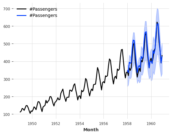
Furthermore, we could also for instance specify that we have some prior belief that the scale of the distribution is about \(0.1\) (in the transformed domain), while still capturing some time dependency of the distribution, by specifying prior_b=.1.
Behind the scenes this will regularize the training loss with a Kullback-Leibler divergence term.
[61]:
model = TCNModel(
    input_chunk_length=24,
    output_chunk_length=12,
    random_state=42,
    likelihood=LaplaceLikelihood(prior_b=0.1),
    pl_trainer_kwargs={"accelerator": "cpu"},
)

model.fit(train_air_scaled, epochs=400, verbose=True);
GPU available: True (mps), used: False
TPU available: False, using: 0 TPU cores
HPU available: False, using: 0 HPUs
/Users/dennisbader/miniconda3/envs/darts/lib/python3.10/site-packages/pytorch_lightning/trainer/setup.py:177: GPU available but not used. You can set it by doing `Trainer(accelerator='gpu')`.

  | Name            | Type             | Params | Mode
-------------------------------------------------------------
0 | criterion       | MSELoss          | 0      | train
1 | train_criterion | MSELoss          | 0      | train
2 | val_criterion   | MSELoss          | 0      | train
3 | train_metrics   | MetricCollection | 0      | train
4 | val_metrics     | MetricCollection | 0      | train
5 | res_blocks      | ModuleList       | 166    | train
-------------------------------------------------------------
166       Trainable params
0         Non-trainable params
166       Total params
0.001     Total estimated model params size (MB)
23        Modules in train mode
0         Modules in eval mode
`Trainer.fit` stopped: `max_epochs=400` reached.
[62]:
pred = model.predict(n=36, num_samples=500)

# scale back:
pred = scaler.inverse_transform(pred, series_idx=0)

series_air.plot()
pred.plot();
GPU available: True (mps), used: False
TPU available: False, using: 0 TPU cores
HPU available: False, using: 0 HPUs
By default TimeSeries.plot() shows the median as well as the 5th and 95th percentiles (of the marginal distributions, if the TimeSeries is multivariate). It is possible to control this:
[63]:
pred.plot(low_quantile=0.01, high_quantile=0.99, label="1-99th percentiles")
pred.plot(low_quantile=0.2, high_quantile=0.8, label="20-80th percentiles");

Types of distributions#
The likelihood has to be compatible with the domain of your time series’ values. For instance PoissonLikelihood can be used on discrete positive values, ExponentialLikelihood can be used on real positive values, and BetaLikelihood on real values in \((0,1)\).
It is also possible to use QuantileRegression to apply a quantile loss and fit some desired quantiles directly.
Evaluating Probabilistic Forecasts#
How can we evaluate the quality of probabilistic forecasts? By default, most metrics functions (such as mape()) will keep working but look only at the median forecast. It is also possible to use the Mean Quantile Loss metric mql(), which quantifies the error for each predicted quantiles. For quantile=0.5 (the median), it is identical to the Mean Absolute Error (MAE):
[64]:
from darts.metrics import mae, mql

print(f"MAPE of median forecast: {mape(series_air, pred):.2f}")
print(f"MAE of median forecast: {mae(series_air, pred):.2f}")
for q in [0.05, 0.1, 0.5, 0.9, 0.95]:
    q_loss = mql(series_air, pred, q=q)
    print(f"quantile loss at quantile {q:.2f}: {q_loss:.2f}")
MAPE of median forecast: 12.14
MAE of median forecast: 51.64
quantile loss at quantile 0.05: 5.33
quantile loss at quantile 0.10: 13.14
quantile loss at quantile 0.50: 51.64
quantile loss at quantile 0.90: 20.74
quantile loss at quantile 0.95: 12.20
Using Quantile Loss#
Could we do better by fitting these quantiles directly? We can just use a QuantileRegression likelihood:
[65]:
from darts.utils.likelihood_models.torch import QuantileRegression

model = TCNModel(
    input_chunk_length=24,
    output_chunk_length=12,
    random_state=42,
    likelihood=QuantileRegression([0.05, 0.1, 0.5, 0.9, 0.95]),
)

model.fit(train_air_scaled, epochs=400, verbose=True);
GPU available: True (mps), used: True
TPU available: False, using: 0 TPU cores
HPU available: False, using: 0 HPUs

  | Name            | Type             | Params | Mode
-------------------------------------------------------------
0 | criterion       | MSELoss          | 0      | train
1 | train_criterion | MSELoss          | 0      | train
2 | val_criterion   | MSELoss          | 0      | train
3 | train_metrics   | MetricCollection | 0      | train
4 | val_metrics     | MetricCollection | 0      | train
5 | res_blocks      | ModuleList       | 208    | train
-------------------------------------------------------------
208       Trainable params
0         Non-trainable params
208       Total params
0.001     Total estimated model params size (MB)
23        Modules in train mode
0         Modules in eval mode
`Trainer.fit` stopped: `max_epochs=400` reached.
[66]:
pred = model.predict(n=36, num_samples=500)

# scale back:
pred = scaler.inverse_transform(pred, series_idx=0)

series_air.plot()
pred.plot()

print(f"MAPE of median forecast: {mape(series_air, pred):.2f}")
for q in [0.05, 0.1, 0.5, 0.9, 0.95]:
    q_loss = mql(series_air, pred, q=q)
    print(f"quantile loss at quantile {q:.2f}: {q_loss:.2f}")
GPU available: True (mps), used: True
TPU available: False, using: 0 TPU cores
HPU available: False, using: 0 HPUs
MAPE of median forecast: 4.91
quantile loss at quantile 0.05: 9.05
quantile loss at quantile 0.10: 13.50
quantile loss at quantile 0.50: 20.07
quantile loss at quantile 0.90: 11.99
quantile loss at quantile 0.95: 7.39
With Regression Models#
Probailistic support for our SKLearnModels is similiar to that of the neural networks. We have to specify a likelihood at model creation. Instead of giving a likelihood object, we can simply pick one of "quantile" (with some quantiles) and "poisson".
[67]:
model = LinearRegressionModel(
    lags=24,
    lags_future_covariates=[0],
    likelihood="quantile",
    quantiles=[0.05, 0.1, 0.5, 0.9, 0.95],
)
model.fit(train_air, future_covariates=air_covs)
pred = model.predict(n=36, num_samples=500)

series_air.plot()
pred.plot()

print(f"MAPE of median forecast: {mape(series_air, pred):.2f}")
for q in [0.05, 0.1, 0.5, 0.9, 0.95]:
    q_loss = mql(series_air, pred, q=q)
    print(f"quantile loss at quantile {q:.2f}: {q_loss:.2f}")
MAPE of median forecast: 8.52
quantile loss at quantile 0.05: 20.76
quantile loss at quantile 0.10: 25.44
quantile loss at quantile 0.50: 35.33
quantile loss at quantile 0.90: 11.15
quantile loss at quantile 0.95: 6.19
Ensembling models#
Ensembling is about combining the forecasts produced by several models, in order to obtain a final - and hopefully better forecast.
For instance, in our example of a less naive model above, we manually combined a naive seasonal model with a naive drift model. Here, we will show how model forecasts can be automatically combined - naively using a NaiveEnsembleModel, or learned using RegressionEnsembleModel.
It is of course also possible to use past and/or future_covariates with ensemble model but they will be passed only to the forecasting models supporting them.
Naive Ensembling#
Naive ensembling just takes the average of the forecasts from several models. Darts NaiveEnsembleModel does exactly that and all through the same API as the forecasting models (fit, predict, historical forecasts, backtesting, …).
[68]:
from darts.models import NaiveEnsembleModel

models = [NaiveDrift(), NaiveSeasonal(12)]

ensemble_model = NaiveEnsembleModel(forecasting_models=models)

backtest = ensemble_model.historical_forecasts(**hfc_params)

print(f"MAPE = {mape(backtest, series_air):.2f}%")
series_air.plot()
backtest.plot();
MAPE = 11.93%

Learned Ensembling#
As expected in this case, the naive ensemble doesn’t give great results (although in some cases it could!)
We can sometimes do better if we see the ensembling as a supervised regression problem: given a set of forecasts (features), find a model that combines them in order to minimise errors on the target. This is what the RegressionEnsembleModel does. It accepts parameters:
forecasting_modelsis a list of forecasting models whose predictions we want to ensemble.regression_train_n_pointsis the number of time steps to use for fitting the “ensemble regression” model (i.e., the inner model that combines the forecasts).regression_modelis, optionally, a sklearn-compatible regression model or a DartsSKLearnModelto be used for the ensemble regression. If not specified, a linear regression is used. Using a sklearn model is easy out-of-the-box, but using aSKLearnModelallows to potentially take arbitrary lags of the individual forecasts as inputs of the regression model.and for more, read our this user guide on ensembling models.
Once these elements are in place, a RegressionEnsembleModel can be used like a regular forecasting model:
[69]:
from darts.models import RegressionEnsembleModel

ensemble_model = RegressionEnsembleModel(
    forecasting_models=models, regression_train_n_points=12
)

backtest = ensemble_model.historical_forecasts(**hfc_params)

print(f"MAPE = {mape(backtest, series_air):.2f}")
series_air.plot()
backtest.plot();
MAPE = 4.77
We can also inspect the coefficients used to weigh the two inner models in the linear combination:
[70]:
ensemble_model.fit(series_air)
ensemble_model.ensemble_model.model.coef_
[70]:
array([0.01368814, 1.0980107 ], dtype=float32)
Ensemble models can also be probabilistic themselves! You can read about it in our guide on ensembling models.
RegressionEnsembleModel uses the stacking technique to train and combine the forecasting_models: each one of them is trained independently and the regression_model is then trained using their predictions as future_covariates.
Filtering models#
In addition to forecasting models, which are able to predict future values of series, Darts also contains a couple of helpful filtering models, which can model “in sample” series’ values distributions.
Fitting a Kalman Filter#
KalmanFilter implements a Kalman Filter. The implementation relies on nfoursid, so it is for instance possible to provide a nfoursid.kalman.Kalman object containing a transition matrix, process noise covariance, observation noise covariance etc.
It is also possible to do system identification by calling fit() to “train” the Kalman Filter using the N4SID system identification algorithm:
[71]:
from darts.models import KalmanFilter

kf = KalmanFilter(dim_x=3)
kf.fit(train_air_scaled)
filtered_series = kf.filter(train_air_scaled, num_samples=100)

train_air_scaled.plot()
filtered_series.plot();
Inferring missing values with Gaussian Processes#
Darts also contains a GaussianProcessFilter which can be used for probabilistic modeling of series:
[72]:
from sklearn.gaussian_process.kernels import RBF

from darts.models import GaussianProcessFilter

# create a series with holes:
values = train_air_scaled.values()
values[20:22] = np.nan
values[28:32] = np.nan
values[55:59] = np.nan
values[72:80] = np.nan
series_holes = TimeSeries.from_times_and_values(train_air_scaled.time_index, values)
series_holes.plot()

kernel = RBF()

gpf = GaussianProcessFilter(kernel=kernel, alpha=0.1, normalize_y=True)
filtered_series = gpf.filter(series_holes, num_samples=100)

filtered_series.plot();
A Word of Caution#
So is N-BEATS, exponential smoothing, or a Bayesian ridge regression trained on milk production the best approach for predicting the future number of airline passengers? Well, at this point it’s actually hard to say exactly which one is best. Our time series is small, and our validation set is even smaller. In such cases, it’s very easy to overfit the whole forecasting exercise to such a small validation set. That’s especially true if the number of available models and their degrees of freedom is high (such as for deep learning models), or if we played with many models on a single test set (as done in this notebook).
As data scientists, it is our responsibility to understand the extent to which our models can be trusted. So always take results with a grain of salt, especially on small datasets, and apply the scientific method before making any kind of forecast :) Happy modeling!
Anomaly Detection#
Darts also has an entire module on Time Series Anomaly Detection. For more info, read our user guide on anomaly detection.
[ ]: