[1]:
# fix python path if working locally
from utils import fix_pythonpath_if_working_locally

fix_pythonpath_if_working_locally()
[2]:
%load_ext autoreload
%autoreload 2
%matplotlib inline
[3]:
import warnings

import matplotlib.pyplot as plt
import numpy as np
import pandas as pd

# use darts plotting style
from darts import set_option

set_option("plotting.use_darts_style", True)

from darts import TimeSeries

warnings.filterwarnings("ignore")
import logging

logging.disable(logging.CRITICAL)
Static Covariates#
Static covariates are characteristics of a time series / constants which do not change over time. When dealing with multiple time series, static covariates can help specific models improve forecasts. Darts’ models will only consider static covariates embedded in the target series (the series for which we want to predict future values) and not past and/or future covariates (external data).
In this tutorial we look at:
how to define static covariates (numeric and/or categorical)
how to add static covariates to an existing target series
how to add static covariates at TimeSeries creation
how to use TimeSeries.from_group_dataframe() for automatic extraction of TimeSeries with embedded static covariates
how to scale/transform/encode static covariates embedded in your series
how to use static covariates with Darts’ models
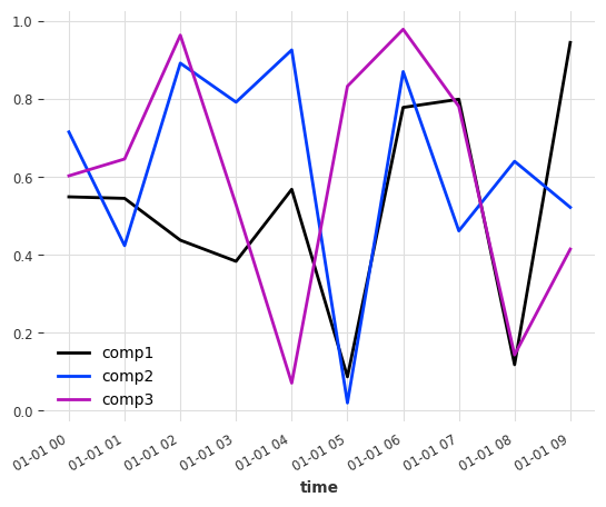
We start by generating a multivariate time series with three components ["comp1", "comp2", "comp3"]
[4]:
np.random.seed(0)
series = TimeSeries.from_times_and_values(
    times=pd.date_range(start="2020-01-01", periods=10, freq="h"),
    values=np.random.random((10, 3)),
    columns=["comp1", "comp2", "comp3"],
)
series.plot()
1. Defining static covariates#
Define your static covariates as a pd.DataFrame where the columns represent the static variables and rows stand for the components of the uni/multivariate TimeSeries they will be added to.
The number of rows must either be 1 or equal to the number of components from
series.Using a single row static covariate DataFrame with a multivariate (multi component)
series, the static covariates will be mapped globally to all components.
[5]:
# arbitrary continuous and categorical static covariates (single row)
static_covs_single = pd.DataFrame(data={"cont": [0], "cat": ["a"]})
print(static_covs_single)

# multivariate static covariates (multiple components).
# note that the number of rows matches the number of components of `series`
static_covs_multi = pd.DataFrame(data={"cont": [0, 2, 1], "cat": ["a", "c", "b"]})
print(static_covs_multi)
   cont cat
0     0   a
   cont cat
0     0   a
1     2   c
2     1   b
2. Add static covariates to an existing TimeSeries#
Create a new series from an existing TimeSeries with added static covariates using method with_static_covariates() (see docs here)
Single row static covarites with multivariate
seriescreates “global_components” which are mapped to all componentsMulti row static covarites with multivariate
serieswill be mapped to the component names ofseries(see static covariate index/row names)
[6]:
assert series.static_covariates is None

series_single = series.with_static_covariates(static_covs_single)
print("Single row static covarites with multivariate `series`")
print(series_single.static_covariates)

series_multi = series.with_static_covariates(static_covs_multi)
print("\nMulti row static covarites with multivariate `series`")
print(series_multi.static_covariates)
Single row static covarites with multivariate `series`
static_covariates  cont cat
global_components   0.0   a

Multi row static covarites with multivariate `series`
static_covariates  cont cat
component
comp1               0.0   a
comp2               2.0   c
comp3               1.0   b
3. Adding static covariates at TimeSeries construction#
Static covariates can also directly be added when creating a time series with parameter static_covariates in most of TimeSeries.from_*() methods.
[7]:
# add arbitrary continuous and categorical static covariates
series = TimeSeries.from_values(
    values=np.random.random((10, 3)),
    columns=["comp1", "comp2", "comp3"],
    static_covariates=static_covs_multi,
)
print(series.static_covariates)
static_covariates  cont cat
component
comp1               0.0   a
comp2               2.0   c
comp3               1.0   b
Using static covariates with multiple TimeSeries#
Static covariates are only really useful if we use them across multiple TimeSeries. By convention, the static covariates layout (pd.DataFrame columns, index) has to be the same for all series.
[8]:
first_series = series.with_static_covariates(
    pd.DataFrame(data={"ID": ["SERIES1"], "var1": [0.5]})
)
second_series = series.with_static_covariates(
    pd.DataFrame(data={"ID": ["SERIES2"], "var1": [0.75]})
)

print("Valid static covariates for multiple series")
print(first_series.static_covariates)
print(second_series.static_covariates)

series_multi = [first_series, second_series]
Valid static covariates for multiple series
static_covariates       ID  var1
global_components  SERIES1   0.5
static_covariates       ID  var1
global_components  SERIES2  0.75
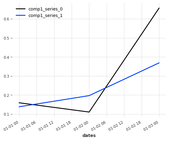
4. Extract a list of time series by groups from a DataFrame using from_group_dataframe()#
If your DataFrame contains multiple time series which are stacked vertically, you can use TimeSeries.from_group_dataframe() (see the docs here) to extract them as a list of TimeSeries instances. This requires a column or list of columns for which the DataFrame should grouped by (parameter group_cols). group_cols will automatically be added as static covariates to
the individual series. Additional columns can be used as static covariates with parameter static_cols.
In the example below, we generate a DataFrame which contains data of two distinct time series (overlapping/repeating dates) “SERIES1” and “SERIES2” and extract the TimeSeries with from_group_dataframe().
[9]:
# generate an DataFrame example
df = pd.DataFrame(
    data={
        "dates": [
            "2020-01-01",
            "2020-01-02",
            "2020-01-03",
            "2020-01-01",
            "2020-01-02",
            "2020-01-03",
        ],
        "comp1": np.random.random((6,)),
        "comp2": np.random.random((6,)),
        "comp3": np.random.random((6,)),
        "ID": ["SERIES1", "SERIES1", "SERIES1", "SERIES2", "SERIES2", "SERIES2"],
        "var1": [0.5, 0.5, 0.5, 0.75, 0.75, 0.75],
    }
)
print("Input DataFrame")
print(df)

series_multi = TimeSeries.from_group_dataframe(
    df,
    time_col="dates",
    group_cols="ID",  # individual time series are extracted by grouping `df` by `group_cols`
    static_cols=[
        "var1"
    ],  # also extract these additional columns as static covariates (without grouping)
    value_cols=[
        "comp1",
        "comp2",
        "comp3",
    ],  # optionally, specify the time varying columns
)

print(f"\n{len(series_multi)} series were extracted from the input DataFrame")
for i, ts in enumerate(series_multi):
    print(f"Static covariates of series {i}")
    print(ts.static_covariates)
    ts["comp1"].plot(label=f"comp1_series_{i}")
Input DataFrame
        dates     comp1     comp2     comp3       ID  var1
0  2020-01-01  0.158970  0.820993  0.976761  SERIES1  0.50
1  2020-01-02  0.110375  0.097101  0.604846  SERIES1  0.50
2  2020-01-03  0.656330  0.837945  0.739264  SERIES1  0.50
3  2020-01-01  0.138183  0.096098  0.039188  SERIES2  0.75
4  2020-01-02  0.196582  0.976459  0.282807  SERIES2  0.75
5  2020-01-03  0.368725  0.468651  0.120197  SERIES2  0.75

2 series were extracted from the input DataFrame
Static covariates of series 0
static_covariates       ID  var1
global_components  SERIES1   0.5
Static covariates of series 1
static_covariates       ID  var1
global_components  SERIES2  0.75
5. Scaling/Encoding/Transforming static covariate data#
There might be the need to scale numeric static covariates or encode categorical static covariates as not all models can handle non numeric static covariates.
Use StaticCovariatesTransformer (see the docs here) to scale/transform static covariates. By default it uses a MinMaxScaler to scale numeric data, and a OrdinalEncoder to encode categorical data. Both the numeric and categorical transformers will be fit globally on static covariate data of all time series passed to
StaticCovariatesTransformer.fit()
[10]:
from darts.dataprocessing.transformers import StaticCovariatesTransformer

transformer = StaticCovariatesTransformer()
series_transformed = transformer.fit_transform(series_multi)

for i, (ts, ts_scaled) in enumerate(zip(series_multi, series_transformed)):
    print(f"Original series {i}")
    print(ts.static_covariates)
    print(f"Transformed series {i}")
    print(ts_scaled.static_covariates)
    print("")
Original series 0
static_covariates       ID  var1
global_components  SERIES1   0.5
Transformed series 0
static_covariates   ID  var1
global_components  0.0   0.0

Original series 1
static_covariates       ID  var1
global_components  SERIES2  0.75
Transformed series 1
static_covariates   ID  var1
global_components  1.0   1.0
6. Forecasting example with TFTModel and static covariates#
Now let’s find out if adding static covariates to a forecasting problem can improve predictive accuracy. We’ll use TFTModel which supports numeric and categorical static covariates.
[11]:
import numpy as np
import pandas as pd
from pytorch_lightning.callbacks import TQDMProgressBar

from darts import TimeSeries
from darts.dataprocessing.transformers import StaticCovariatesTransformer
from darts.metrics import rmse
from darts.models import TFTModel
from darts.utils import timeseries_generation as tg
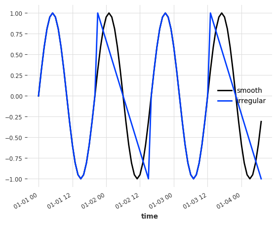
6.1 Experiment setup#
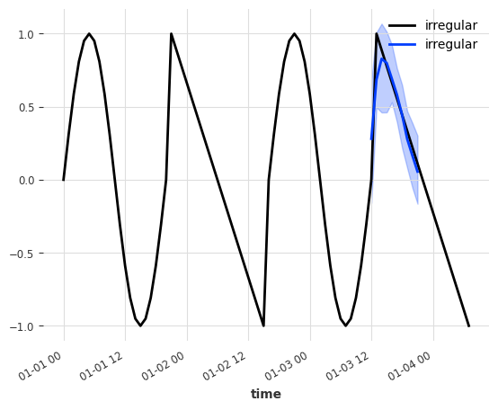
For our experiment, we generate two time series: a fully sine wave series (label = smooth) and sine wave series with some irregularities every other period (label = irregular, see the ramps at periods 2 and 4).
[12]:
period = 20
sine_series = tg.sine_timeseries(
    length=4 * period, value_frequency=1 / period, column_name="smooth", freq="h"
)

sine_vals = sine_series.values()
linear_vals = np.expand_dims(np.linspace(1, -1, num=19), -1)

sine_vals[21:40] = linear_vals
sine_vals[61:80] = linear_vals
irregular_series = TimeSeries.from_times_and_values(
    values=sine_vals, times=sine_series.time_index, columns=["irregular"]
)
sine_series.plot()
irregular_series.plot()
We will use three different setups for training and evaluation:
fit/predict without static covariates
fit/predict with binary (numeric) static covariates
fit/predict with categorical static covariates
For each setup we’ll train the model on both series and then only use only the 3rd period (sine wave for both series) to predict the 4th period (sine for “smooth” and ramp for “irregular”).
What we hope for is that the model without static covariates performs worse than the other ones. The non-static model should not be able to recognize whether the underlying series used in predict() is the smooth or the irregular series as it only gets a sine wave curve as input (3rd period). This should result in a forecast somewhere inbetween the smooth and irregular series (learned by minimizing the global loss during training).
Now this is where static covariates can really help. For example, we can embed data about the curve type into the target series through static covariates. With this information, we’d expect the models to generate improved forecasts.
First we create some helper functions to apply the same experiment conditions to all models.
[13]:
def test_case(model, train_series, predict_series):
    """helper function which performs model training, prediction and plotting"""
    model.fit(train_series)
    preds = model.predict(n=int(period / 2), num_samples=250, series=predict_series)
    for ts, ps in zip(train_series, preds):
        ts.plot()
        ps.plot()
        plt.show()
    return preds


def get_model_params():
    """helper function that generates model parameters with a new Progress Bar object"""
    return {
        "input_chunk_length": int(period / 2),
        "output_chunk_length": int(period / 2),
        "add_encoders": {
            "datetime_attribute": {"future": ["hour"]}
        },  # TFTModel requires future input, with this we won't have to supply any future_covariates
        "random_state": 42,
        "n_epochs": 150,
        "pl_trainer_kwargs": {
            "callbacks": [TQDMProgressBar(refresh_rate=4)],
        },
    }
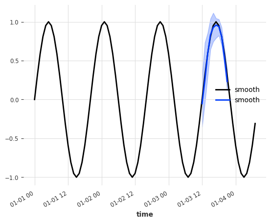
6.2 Forecasting without static covariates#
Let’s train the first model without any static covariates
[14]:
train_series = [sine_series, irregular_series]
for series in train_series:
    assert not series.has_static_covariates

model = TFTModel(**get_model_params())
preds = test_case(
    model,
    train_series,
    predict_series=[series[:60] for series in train_series],
)
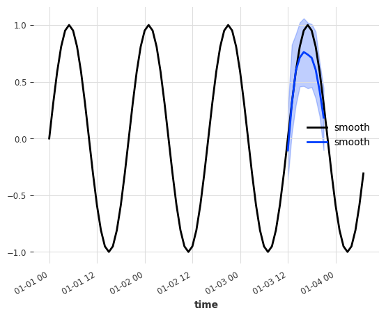
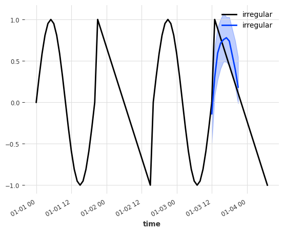
From the plot you can see that the forecast began after period 3 (~01-03-2022 - 12:00). The prediciton input were the last input_chunk_length=10 values - which are identical for both series (sine wave).
As expected, the model was not able to determine the type of the underlying prediciton series (smooth or irregular) and generate a sine-wave like forecast for both.
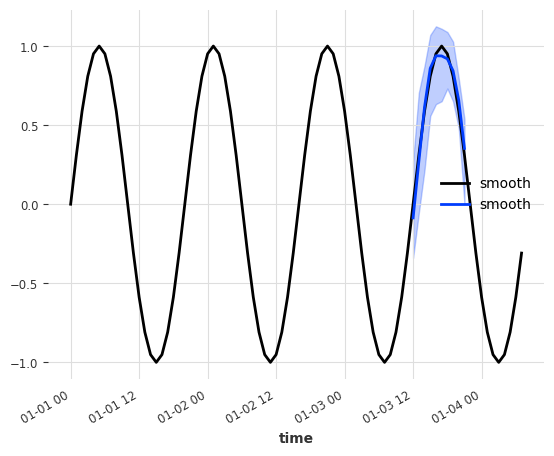
6.3 Forecasting with 0/1 binary static covariates (numeric)#
Now let’s repeat the experiment but this time we add information about the curve type as a binary (numeric) static covariate named "curve_type".
[15]:
sine_series_st_bin = sine_series.with_static_covariates(
    pd.DataFrame(data={"curve_type": [1]})
)
irregular_series_st_bin = irregular_series.with_static_covariates(
    pd.DataFrame(data={"curve_type": [0]})
)

train_series = [sine_series_st_bin, irregular_series_st_bin]
for series in train_series:
    print(series.static_covariates)

model = TFTModel(**get_model_params())
preds_st_bin = test_case(
    model,
    train_series,
    predict_series=[series[:60] for series in train_series],
)
static_covariates  curve_type
component
smooth                    1.0
static_covariates  curve_type
component
irregular                 0.0
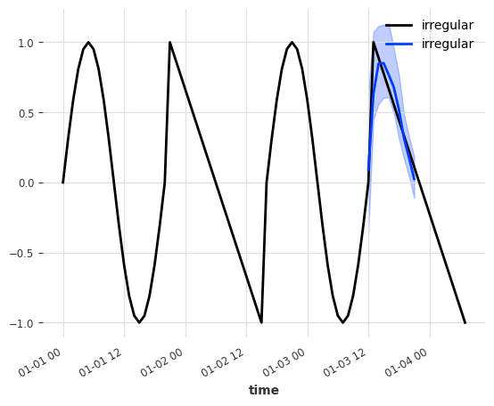
That already looks much better! The model was able to identify the curve type/category from the binary static covariate feature.
6.4 Forecasting with categorical static covariates#
The last experiment already showed promising results. So why not only use binary features for categorical data? While it might have worked well for our two time series, if we had more curve types we’d need to one hot encode the feature into a binary variable for each category. With a lot of categories, this lead to a large number of features/predictors and multicollinearity which can lower the model’s predictive accuracy.
As a last experiment, let’s use the curve type as a categorical feature. TFTModel learns an embedding for categorical features. Darts’ TorchForecastingModels (such as TFTModel) only support numeric data. Before training we need to transform the "curve_type" into a integer-valued feature with StaticCovariatesTransformer (see section 5.).
[16]:
sine_series_st_cat = sine_series.with_static_covariates(
    pd.DataFrame(data={"curve_type": ["smooth"]})
)
irregular_series_st_cat = irregular_series.with_static_covariates(
    pd.DataFrame(data={"curve_type": ["non_smooth"]})
)

train_series = [sine_series_st_cat, irregular_series_st_cat]
print("Static covariates before encoding:")
print(train_series[0].static_covariates)

# use StaticCovariatesTransformer to encode categorical static covariates into numeric data
scaler = StaticCovariatesTransformer()
train_series = scaler.fit_transform(train_series)
print("\nStatic covariates after encoding:")
print(train_series[0].static_covariates)
Static covariates before encoding:
static_covariates curve_type
component
smooth                smooth

Static covariates after encoding:
static_covariates  curve_type
component
smooth                    1.0
No all we need to do is tell TFTModel that "curve_type" is a categorical variable that requires embedding. We can do so with model parameter categorical_embedding_sizes which is a dictionary of: {feature name: (number of categories, embedding size)}
[17]:
n_categories = 2  # "smooth" and "non_smooth"
embedding_size = 2  # embed the categorical variable into a numeric vector of size 2
categorical_embedding_sizes = {"curve_type": (n_categories, embedding_size)}

model = TFTModel(
    categorical_embedding_sizes=categorical_embedding_sizes, **get_model_params()
)
preds_st_cat = test_case(
    model,
    train_series,
    predict_series=[series[:60] for series in train_series],
)
Nice, that seems to have worked as well! As a last step, let’s look at how the models performed compared to each other.
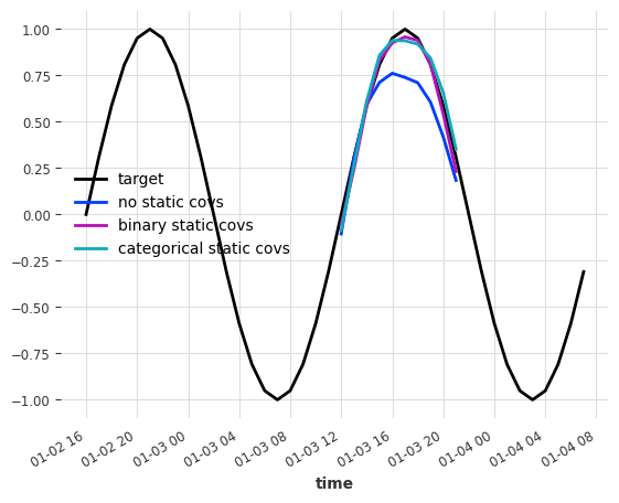
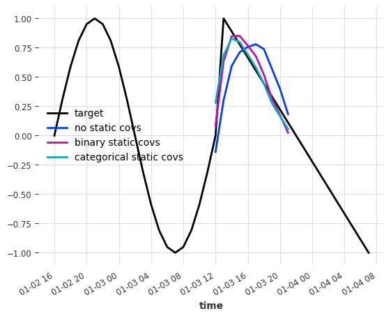
[18]:
for series, ps_no_st, ps_st_bin, ps_st_cat in zip(
    train_series, preds, preds_st_bin, preds_st_cat
):
    series[-40:].plot(label="target")
    ps_no_st.quantile(0.5).plot(label="no static covs")
    ps_st_bin.quantile(0.5).plot(label="binary static covs")
    ps_st_cat.quantile(0.5).plot(label="categorical static covs")
    plt.show()
    print("Metric")
    print(
        pd.DataFrame(
            {
                name: [rmse(series, ps)]
                for name, ps in zip(
                    ["no st", "bin st", "cat st"], [ps_no_st, ps_st_bin, ps_st_cat]
                )
            },
            index=["RMSE"],
        )
    )
Metric
        no st    bin st    cat st
RMSE  0.16352  0.042527  0.050242
Metric
         no st    bin st    cat st
RMSE  0.289051  0.138122  0.138631
These are great results! Both approaches using static covariates decreased the RMSE by more than halve for both series compared to the baseline!
Note that we only used one static covariate feature, but you can use as many as want including mixtures of data types (numeric and categorical).