Temporal Fusion Transformer#
In this notebook, we show two examples of how two use Darts’ TFTModel. If you are new to darts, we recommend you first follow the quick start notebook.
[1]:
# fix python path if working locally
from utils import fix_pythonpath_if_working_locally

fix_pythonpath_if_working_locally()
[2]:
%load_ext autoreload
%autoreload 2
%matplotlib inline
[ ]:
# use darts plotting style
from darts import set_option

set_option("plotting.use_darts_style", True)
[3]:
import warnings

import matplotlib.pyplot as plt
import numpy as np
import pandas as pd

from darts import TimeSeries, concatenate
from darts.dataprocessing.transformers import Scaler
from darts.datasets import AirPassengersDataset, IceCreamHeaterDataset
from darts.metrics import mape
from darts.models import TFTModel
from darts.utils.likelihood_models.torch import QuantileRegression
from darts.utils.statistics import check_seasonality, plot_acf
from darts.utils.timeseries_generation import datetime_attribute_timeseries

warnings.filterwarnings("ignore")
import logging

logging.disable(logging.CRITICAL)
Temporal Fusion Transformer (TFT)#
Darts’ TFTModel incorporates the following main components from the original Temporal Fusion Transformer (TFT) architecture as outlined in this paper:
gating mechanisms: skip over unused components of the model architecture
variable selection networks: select relevant input variables at each time step.
temporal processing of past and future input with LSTMs (long short-term memory)
multi-head attention: captures long-term temporal dependencies
prediction intervals: per default, produces quantile forecasts instead of deterministic values
Training#
TFTModel can be trained with past and future covariates. It is trained sequentially on fixed-size chunks consisting of an encoder and a decoder part:
encoder: past input with
input_chunk_lengthpast target: mandatory
past covariates: optional
decoder: future known input with
output_chunk_lengthfuture covariates: mandatory (if none are available, consider
TFTModel’s optional argumentsadd_encodersoradd_relative_indexfrom here)
In each iteration, the model produces a quantile prediction of shape (output_chunk_length, n_quantiles) on the decoder part.
Forecast#
Probabilistic Forecast#
Per default, TFTModel produces probabilistic quantile forecasts using QuantileRegression. This gives the range of likely target values at each prediction step. Most deep learning models in Darts’ - including TFTModel - support QuantileRegression and 16 other likelihoods to produce probabilistic forecasts by setting likelihood=MyLikelihood() at model creation.
To produce meaningful results, set num_samples >> 1 when predicting. For example:
model.predict(*args, **kwargs, num_samples=200)
Predictions with forecasting horizon n are generated auto-regressively using encoder-decoder chunks of the same size as during training.
If n > output_chunk_length, you have to supply additional future values for the covariates you passed to model.train().
Deterministic Forecast#
To produce deterministic rather than probabilistic forecasts, set parameter likelihood to None and loss_fn to a PyTorch loss function at model creation. For example:
model = TFTModel(*args, **kwargs, likelihood=None, loss_fn=torch.nn.MSELoss())
...
model.predict(*args, **kwargs, num_samples=1)
[4]:
# before starting, we define some constants
num_samples = 200

figsize = (9, 6)
lowest_q, low_q, high_q, highest_q = 0.01, 0.1, 0.9, 0.99
label_q_outer = f"{int(lowest_q * 100)}-{int(highest_q * 100)}th percentiles"
label_q_inner = f"{int(low_q * 100)}-{int(high_q * 100)}th percentiles"
Air Passenger Example#
This data set that is highly dependent on covariates. Knowing the month tells us a lot about the seasonal component, whereas the year determines the effect of the trend component.
Additionally, let’s convert the time index to integer values and use them as covariates as well.
All of the three covariates are known in the future, and can be used as future_covariates with the TFTModel.
[5]:
# Read data
series = AirPassengersDataset().load()

# we convert monthly number of passengers to average daily number of passengers per month
series = series / TimeSeries.from_values(series.time_index.days_in_month)
series = series.astype(np.float32)

# Create training and validation sets:
training_cutoff = pd.Timestamp("19571201")
train, val = series.split_after(training_cutoff)

# Normalize the time series (note: we avoid fitting the transformer on the validation set)
transformer = Scaler()
train_transformed = transformer.fit_transform(train)
val_transformed = transformer.transform(val)
series_transformed = transformer.transform(series)

# create year, month and integer index covariate series
covariates = datetime_attribute_timeseries(series, attribute="year", one_hot=False)
covariates = covariates.stack(
    datetime_attribute_timeseries(series, attribute="month", one_hot=False)
)
covariates = covariates.stack(
    TimeSeries.from_times_and_values(
        times=series.time_index,
        values=np.arange(len(series)),
        columns=["linear_increase"],
    )
)
covariates = covariates.astype(np.float32)

# transform covariates (note: we fit the transformer on train split and can then transform the entire covariates series)
scaler_covs = Scaler()
cov_train, cov_val = covariates.split_after(training_cutoff)
scaler_covs.fit(cov_train)
covariates_transformed = scaler_covs.transform(covariates)
Create a model#
If you want to produce deterministic forecasts rather than quantile forecasts, you can use a PyTorch loss function (i.e., set loss_fn=torch.nn.MSELoss() and likelihood=None).
The TFTModel can only be used if some future input is given. Optional parameters add_encoders and add_relative_index can be useful, especially if we don’t have any future input available. They generate encoded temporal data that is used as future covariates.
Since we already have future covariates defined in our example they are commented out.
[6]:
# default quantiles for QuantileRegression
quantiles = [
    0.01,
    0.05,
    0.1,
    0.15,
    0.2,
    0.25,
    0.3,
    0.4,
    0.5,
    0.6,
    0.7,
    0.75,
    0.8,
    0.85,
    0.9,
    0.95,
    0.99,
]
input_chunk_length = 24
forecast_horizon = 12
my_model = TFTModel(
    input_chunk_length=input_chunk_length,
    output_chunk_length=forecast_horizon,
    hidden_size=64,
    lstm_layers=1,
    num_attention_heads=4,
    dropout=0.1,
    batch_size=16,
    n_epochs=300,
    add_relative_index=False,
    add_encoders=None,
    likelihood=QuantileRegression(
        quantiles=quantiles
    ),  # QuantileRegression is set per default
    # loss_fn=MSELoss(),
    random_state=42,
)
Train the TFT#
In what follows, we can just provide the whole covariates series as future_covariates argument to the model; the model will slice these covariates and use only what it needs in order to train on forecasting the target train_transformed:
[7]:
my_model.fit(train_transformed, future_covariates=covariates_transformed, verbose=True)
[7]:
TFTModel(hidden_size=64, lstm_layers=1, num_attention_heads=4, full_attention=False, feed_forward=GatedResidualNetwork, dropout=0.1, hidden_continuous_size=8, categorical_embedding_sizes=None, add_relative_index=False, loss_fn=None, likelihood=<darts.utils.likelihood_models.torch.QuantileRegression object at 0x7f92e0d64c70>, norm_type=LayerNorm, use_static_covariates=True, input_chunk_length=24, output_chunk_length=12, batch_size=16, n_epochs=300, add_encoders=None, random_state=42)
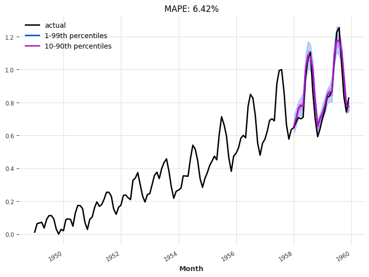
Look at predictions on the validation set#
We perform a one-shot prediction of 24 months using the “current” model - i.e., the model at the end of the training procedure:
[8]:
def eval_model(model, n, actual_series, val_series):
    pred_series = model.predict(n=n, num_samples=num_samples)

    # plot actual series
    plt.figure(figsize=figsize)
    actual_series[: pred_series.end_time()].plot(label="actual")

    # plot prediction with quantile ranges
    pred_series.plot(
        low_quantile=lowest_q, high_quantile=highest_q, label=label_q_outer
    )
    pred_series.plot(low_quantile=low_q, high_quantile=high_q, label=label_q_inner)

    plt.title(f"MAPE: {mape(val_series, pred_series):.2f}%")
    plt.legend()


eval_model(my_model, 24, series_transformed, val_transformed)
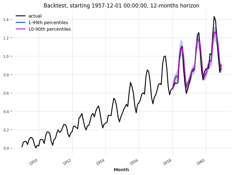
Backtesting#
Let’s backtest our TFTModel model, to see how it performs with a forecast horizon of 12 months over the last 3 years:
[9]:
backtest_series = my_model.historical_forecasts(
    series_transformed,
    future_covariates=covariates_transformed,
    start=train.end_time() + train.freq,
    num_samples=num_samples,
    forecast_horizon=forecast_horizon,
    stride=forecast_horizon,
    last_points_only=False,
    retrain=False,
    verbose=True,
)
[10]:
def eval_backtest(backtest_series, actual_series, horizon, start, transformer):
    plt.figure(figsize=figsize)
    actual_series.plot(label="actual")
    backtest_series.plot(
        low_quantile=lowest_q, high_quantile=highest_q, label=label_q_outer
    )
    backtest_series.plot(low_quantile=low_q, high_quantile=high_q, label=label_q_inner)
    plt.legend()
    plt.title(f"Backtest, starting {start}, {horizon}-months horizon")
    print(
        "MAPE: {:.2f}%".format(
            mape(
                transformer.inverse_transform(actual_series),
                transformer.inverse_transform(backtest_series),
            )
        )
    )


eval_backtest(
    backtest_series=concatenate(backtest_series),
    actual_series=series_transformed,
    horizon=forecast_horizon,
    start=training_cutoff,
    transformer=transformer,
)
MAPE: 4.90%
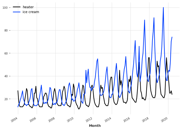
Monthly ice cream sales#
Let’s try a another data set. That of monthly ice cream and heater sales since 2004. Our target is to predict future ice cream sales. First, we build the time series from the data, and check its periodicity.
[11]:
series_ice_heater = IceCreamHeaterDataset().load().astype(np.float32)

plt.figure(figsize=figsize)
series_ice_heater.plot()

print(check_seasonality(series_ice_heater["ice cream"], max_lag=36))
print(check_seasonality(series_ice_heater["heater"], max_lag=36))

plt.figure(figsize=figsize)
plot_acf(series_ice_heater["ice cream"], 12, max_lag=36)  # ~1 year seasonality
(True, 12)
(True, 12)
<Figure size 900x600 with 0 Axes>
Process the data#
We again have a 12-month seasonality. This time we will not define monthly future covariates -> we let the model handle this itself!
Let’s define past covariates instead. What if we used past data of heater sales to predict ice cream sales?
[12]:
# convert monthly sales to average daily sales per month
converted_series = []
for col in ["ice cream", "heater"]:
    converted_series.append(
        series_ice_heater[col]
        / TimeSeries.from_values(series_ice_heater.time_index.days_in_month)
    )
converted_series = concatenate(converted_series, axis=1)
converted_series = converted_series[pd.Timestamp("20100101") :]

# define train/validation cutoff time
forecast_horizon_ice = 12
training_cutoff_ice = converted_series.time_index[-(2 * forecast_horizon_ice)]

# use ice cream sales as target, create train and validation sets and transform data
series_ice = converted_series["ice cream"]
train_ice, val_ice = series_ice.split_before(training_cutoff_ice)
transformer_ice = Scaler()
train_ice_transformed = transformer_ice.fit_transform(train_ice)
val_ice_transformed = transformer_ice.transform(val_ice)
series_ice_transformed = transformer_ice.transform(series_ice)

# use heater sales as past covariates and transform data
covariates_heat = converted_series["heater"]
cov_heat_train, cov_heat_val = covariates_heat.split_before(training_cutoff_ice)
transformer_heat = Scaler()
transformer_heat.fit(cov_heat_train)
covariates_heat_transformed = transformer_heat.transform(covariates_heat)
Create a model with automatically generated future covariates and train it#
Since we don’t have future covariates defined, we need tell the model to generate future covariates itself.
add_encoders: can add multiple encodings as past and / or future covariates from datetime attributes, cyclic repeating temporal patterns, index positions and customm functions for index encodings. You can even add a transformer that handles proper scaling of the training, validation and prediction data! Read more about it in theTFTModeldocs from hereadd_relative_index: adds a scaled integer position relative to the prediction point for each encoder-decoder chunk (this might be useful if you really don’t want to use any future covariates. The position values remain constant over all chunks and do not add additional information).
We use add_encoders={'cyclic': {'future': ['month']}} to account for the 12-month seasonality as a future covariate..
[13]:
# use the last 3 years as past input data
input_chunk_length_ice = 36

# use `add_encoders` as we don't have future covariates
my_model_ice = TFTModel(
    input_chunk_length=input_chunk_length_ice,
    output_chunk_length=forecast_horizon_ice,
    hidden_size=32,
    lstm_layers=1,
    batch_size=16,
    n_epochs=300,
    dropout=0.1,
    add_encoders={"cyclic": {"future": ["month"]}},
    add_relative_index=False,
    optimizer_kwargs={"lr": 1e-3},
    random_state=42,
)

# fit the model with past covariates
my_model_ice.fit(
    train_ice_transformed, past_covariates=covariates_heat_transformed, verbose=True
)
[13]:
TFTModel(hidden_size=32, lstm_layers=1, num_attention_heads=4, full_attention=False, feed_forward=GatedResidualNetwork, dropout=0.1, hidden_continuous_size=8, categorical_embedding_sizes=None, add_relative_index=False, loss_fn=None, likelihood=None, norm_type=LayerNorm, use_static_covariates=True, input_chunk_length=36, output_chunk_length=12, batch_size=16, n_epochs=300, add_encoders={'cyclic': {'future': ['month']}}, optimizer_kwargs={'lr': 0.001}, random_state=42)
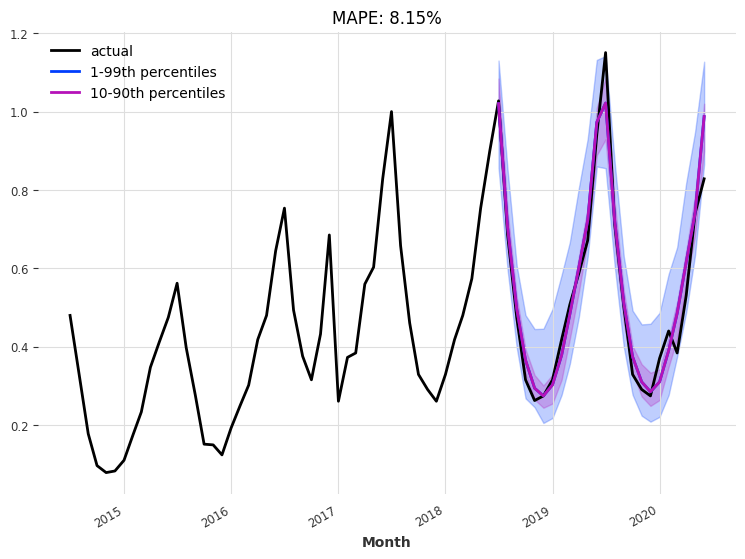
Look at predictions on the validation set#
Again, we perform a one-shot prediction of 24 months using the “current” model - i.e., the model at the end of the training procedure:
[14]:
n = 24
eval_model(
    model=my_model_ice,
    n=n,
    actual_series=series_ice_transformed[
        train_ice.end_time() - (2 * n - 1) * train_ice.freq :
    ],
    val_series=val_ice_transformed,
)
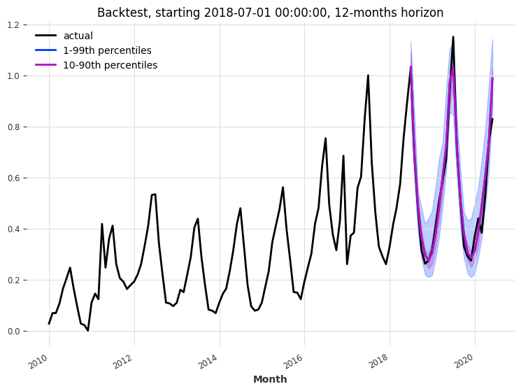
Backtesting#
Let’s backtest our TFTModel model, to see how it performs with a forecast horizon of 12 months over the last 2 years:
[15]:
# Compute the backtest predictions with the two models
last_points_only = False
backtest_series_ice = my_model_ice.historical_forecasts(
    series_ice_transformed,
    num_samples=num_samples,
    start=training_cutoff_ice,
    forecast_horizon=forecast_horizon_ice,
    stride=1 if last_points_only else forecast_horizon_ice,
    retrain=False,
    last_points_only=last_points_only,
    overlap_end=True,
    verbose=True,
)

backtest_series_ice = (
    concatenate(backtest_series_ice)
    if isinstance(backtest_series_ice, list)
    else backtest_series_ice
)
[16]:
eval_backtest(
    backtest_series=backtest_series_ice,
    actual_series=series_ice_transformed[
        train_ice.start_time() - 2 * forecast_horizon_ice * train_ice.freq :
    ],
    horizon=forecast_horizon_ice,
    start=training_cutoff_ice,
    transformer=transformer_ice,
)
MAPE: 5.32%
Explainability#
Let’s try to understand what our TFTModel model has learned. It would be nice to see the feature importance and how much the model attentds to past and future input.
The TFTExplainer does exactly that! You can find the documentation here.
[17]:
from darts.explainability import TFTExplainer
To instantiate the explainer we have two options:
pass a custom background series input to be used as the default input for explanation.
let the explainer load the background from the model automatically. This is only possible if the model was trained on a single target series (as in our case).
[18]:
explainer = TFTExplainer(my_model_ice)
Now we can generate the explanations with explain(). For this we again have two options:
pass a custom foreground series input to be explained
don’t pass any foreground to explain the background
[19]:
explainability_result = explainer.explain()
Let’s look at the feature importances:
encoder feature importance: contains past target, past covariates and “historic” future covariates (the values of future covariates in the input chunk)
decoder fetaure importance: contains “future” future covariates (the values of future covariates in the output chunk)
static covariates importance: the importances of the static variables (only displayed if the model was trained on
serieswith static covariates)
[20]:
explainer.plot_variable_selection(explainability_result);
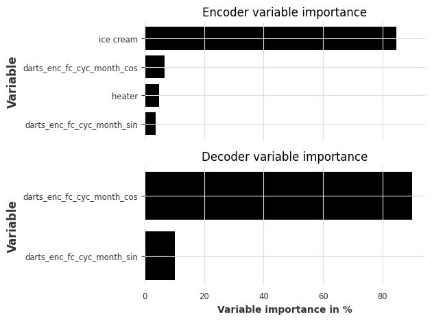
As expected, the past history of ice cream sales is the most important feature in the encoder. The cyclic encoding of the month also helped in the encoder and decoder to learn seasonal patterns.
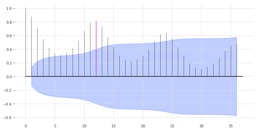
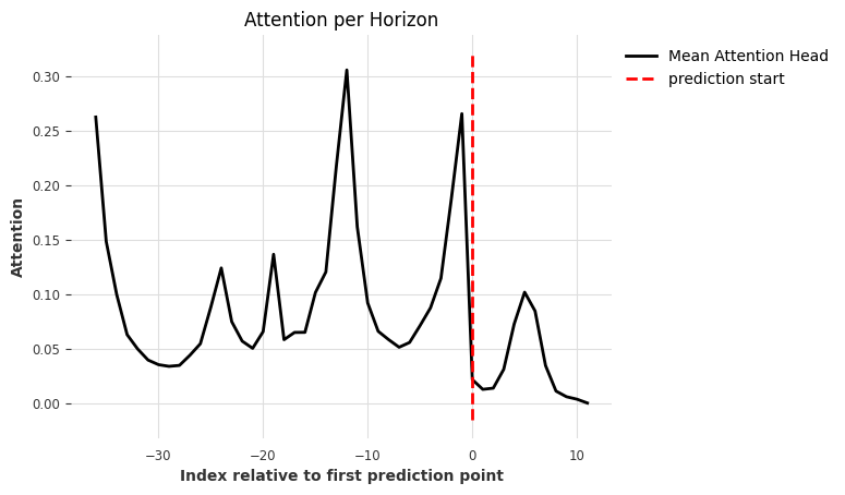
Let’s look at the attention (weights) that the model put on past and future input.
We have multiple plotting options:
plot_type
“time” - plots the attention aggregated over all predictions steps
“all” - plots the attention for each prediction step individually (ranges from
1untiloutput_chunk_length)“heatmap” - plots all the attention for each prediction step as a heatmap
show_index_as
“relative” - sets the x-axis relative to the first predicted time step, ranging from
-input_chunk_lengthuntiloutput_chunk_length - 1.0indicates the first predicted time step (highlighted by a dashed line).“time” - Uses the actual time index on the x-axis. The dashed line highlights the first predicted time step.
[21]:
explainer.plot_attention(explainability_result, plot_type="time");
[21]:
<Axes: title={'center': 'Attention per Horizon'}, xlabel='Index relative to first prediction point', ylabel='Attention'>
We can see interesting attention areas:
maximum attention at relative index -12. This indicates a yearly seasonality which makes sense for ice cream sales.
high attention at the start (-36) of the input chunk: this is probably both from catching the value range of current input and the seasonality (-3 years)
higher attention towards the end (-1) of the input chunk: the model puts attention on the recent past
attention on future input (we look at this more in the next plot)
[22]:
explainer.plot_attention(explainability_result, plot_type="all");
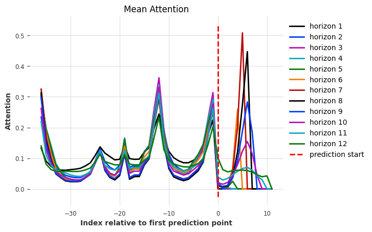
[22]:
<Axes: title={'center': 'Mean Attention'}, xlabel='Index relative to first prediction point', ylabel='Attention'>
On the output chunk (index 0 - 11), we see that the model only attends to the past relative of each horizon. This is because TFTModel uses full_attention=False by default. When setting this to True, the model will also attend to current, and future input.
[23]:
explainer.plot_attention(explainability_result, plot_type="heatmap");

[23]:
<Axes: title={'center': 'Attention Heat Map'}, xlabel='Index relative to first prediction point', ylabel='Horizon'>
We can also get the values directly from the exlainability_result. You can find the documentation here.
[24]:
explainability_result.get_encoder_importance()
[24]:
| darts_enc_fc_cyc_month_sin | heater | darts_enc_fc_cyc_month_cos | ice cream | |
|---|---|---|---|---|
| 0 | 3.7 | 4.8 | 6.8 | 84.7 |
[25]:
explainability_result.get_decoder_importance()
[25]:
| darts_enc_fc_cyc_month_sin | darts_enc_fc_cyc_month_cos | |
|---|---|---|
| 0 | 10.2 | 89.8 |
[26]:
explainability_result.get_static_covariates_importance()
[26]:
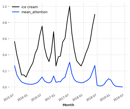
We can also extract the attention as a TimeSeries, and plot it against the data.
[27]:
attention = explainability_result.get_attention().mean(axis=1)

time_intersection = train_ice_transformed.time_index.intersection(attention.time_index)

train_ice_transformed[time_intersection].plot()
attention.plot(label="mean_attention", max_nr_components=12)
Some more information#
Although we have only looked at a single univariate forecasting example, the TFTExplainer can be seemlessly applied to multivariate and / or multiple TimeSeries use cases.