Regression Models
The following is a in depth demonstration of the regression models in Darts - from basic to advanced features, including:
Darts’ regression models
lags and lagged data extraction
covariates usage
parameters output_chunk_length in relation with multi_models
one-shot and auto-regressive predictions
multi output support
probablistic forecasting
explainability
and more
[1]:
# fix python path if working locally
from utils import fix_pythonpath_if_working_locally

fix_pythonpath_if_working_locally()

# activate javascript
from shap import initjs

initjs()
Using `tqdm.autonotebook.tqdm` in notebook mode. Use `tqdm.tqdm` instead to force console mode (e.g. in jupyter console)

[2]:
%load_ext autoreload
%autoreload 2
%matplotlib inline
import matplotlib.pyplot as plt
import numpy as np
import pandas as pd
from sklearn.linear_model import BayesianRidge

from darts.datasets import ElectricityConsumptionZurichDataset
from darts.explainability import ShapExplainer
from darts.metrics import mape
from darts.models import (
    CatBoostModel,
    LightGBMModel,
    LinearRegressionModel,
    RegressionModel,
    XGBModel,
)
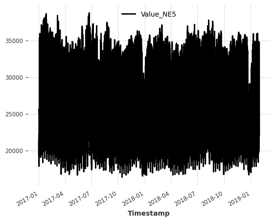
Input Dataset
For this notebook, we use the Electricity Consumption Dataset from households in Zurich, Switzerland.
The dataset has a quarter-hourly frequency (15 Min time intervals), but we resample it to hourly frequency to keep things simple.
Target series (the series we want to forecast): - Value_NE5: Electricity consumption by households on grid level 5 (in kWh).
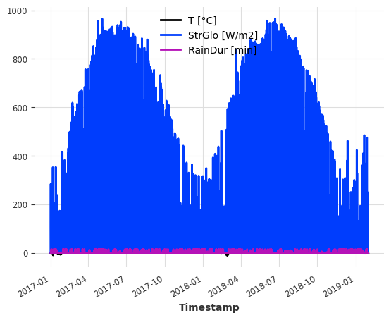
Covariates (external data to help improve forecasts): The dataset also comes with weather measurements that we can use as covariates. For simplicity, we use: - T [°C]: Measured temperature - StrGlo [W/m2]: Measured solar irradation - RainDur [min]: Measured raining duration
[3]:
ts_energy = ElectricityConsumptionZurichDataset().load()

# extract values recorded between 2017 and 2019
start_date = pd.Timestamp("2017-01-01")
end_date = pd.Timestamp("2019-01-31")
ts_energy = ts_energy[start_date:end_date]

# resample to hourly frequency
ts_energy = ts_energy.resample(freq="H")

# extract temperature, solar irradiation and rain duration
ts_weather = ts_energy[["T [°C]", "StrGlo [W/m2]", "RainDur [min]"]]

# extract households energy consumption
ts_energy = ts_energy["Value_NE5"]

# create train and validation splits
validation_cutoff = pd.Timestamp("2018-10-31")
ts_energy_train, ts_energy_val = ts_energy.split_after(validation_cutoff)

ts_energy.plot()
plt.show()

ts_weather.plot()
plt.show()
Darts Regression Models
Regression is a statistical method used in data science and machine learning to model the relationship between a dependent variable (target y) and one or more independent variables (features X).
For convenience, the core Darts package ships with a couple of regression models: - LinearRegressionModel and RandomForest: fully integrated sklearn models - RegressionModel: wrap the Darts Model API around any sklearn-like model - XGBModel: wrapper around XGBoost’s XGBRegressor
In addition to these, we also offer a unified API for some state of the art regression models that can be installed following our installation guide:
LightGBMModel: wrapper around LightGBM’sLightGBMRegressorCatBoostModel: wrapper around CatBoost’sCatBoostRegressor.
In Darts, the forecasting problem is translated into a regression problem by converting the time series into two tabular arrays: - X: features or input array with the shape (number of samples/observations, number of features) - The number of features is given by the total number of (feature specific) target, past, and future covariates lags. - y: target or label array with the shape (number of samples/observations, number of targets) - The number of targets is given by the model
parameters output_chunk_length and multi_models (we’ll explain this later on).
Target and covariates lags
A lagged feature is the value of a feature at a previous or future time step compared to some reference point.
In Darts, the value of the lag specifies the position of the feature value relative to the first predicted target time step y_t0 for each observation/sample (a row in X).
lag == 0: position of the first predicted time stept0, e.g. position ofy_t0lag < 0: all positions in the past of the first predicted time stept-1,t-2, …lag > 0: all positions in the future of the first predicted time stept+1,t+2, …
The choice of lags is critical in achieving good predictive accuracy. We want the model to receive relevant information to capture the temporal properties/dependencies our target series (patterns, seasonalities, trends, …). It also has a considerable impact on the model performance/complexity, as each additional lag adds a new feature to X.
At model creation, we can set lags for the target and the covariates series separately.
lags: lags for the target series (the one we want to forecast)lags_past_covariates: optionally, lags for a past covariates series (external past-observed features to help improve forecasts)lags_future_covariates: optionally, lags for a future covariates series (external future-known features to help improve forecasts)
There are multiple ways to define your lags (int, List[int], Tuple[int, int], ...). You can find out more about this in the RegressionModel docs.
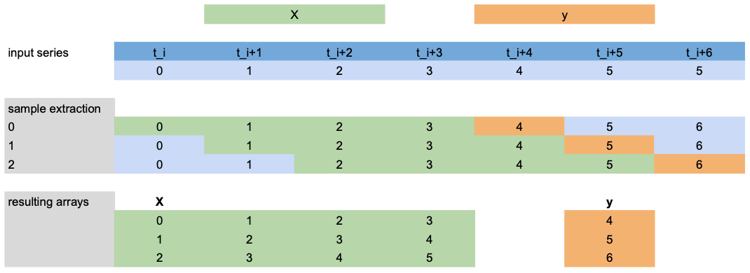
Lagged data extraction
Now, let’s have a look at how X and y is extracted for training using the scenario from below:
lags=[-4,-3,-2,-1]: use the last 4 target values (green) before the first predicted time step (orange) asXfeatures.output_chunk_length=1: predict the target valueyof next (1) time step (orange).we have a target series with 7 time steps
t_i, ..., t_i+6(blue).
Note: This example only shows target ``lags`` extraction, but the same is applied to ``lags_past/future_covariates``.
Examples
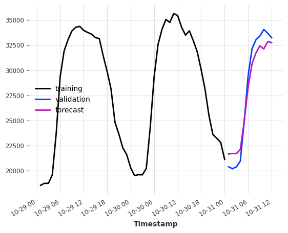
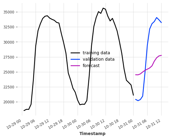
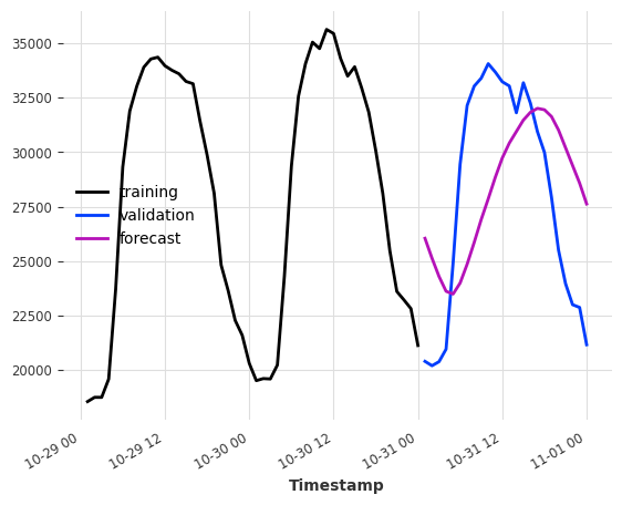
Let’s try to apply this to our electricity dataset. Assume, we want to predict the consumption of the next couple of hours after the end of our training set.
As input features we give it the consumption at the same hour from one and two days ago -> lags=[-24, -48].
[4]:
model = LinearRegressionModel(lags=[-24, -48])
model.fit(ts_energy_train)
pred = model.predict(12)

ts_energy_train[-48:].plot(label="training")
ts_energy_val[:12].plot(label="validation")
pred.plot(label="forecast")
[4]:
<Axes: xlabel='Timestamp'>
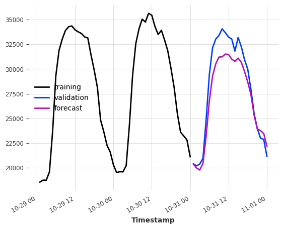
Covariates-based forecasting
To use external data next to the history of our target series, we specify past and/or future covariates lags and then pass past_covariates and/or future_covariates to fit() and predict().
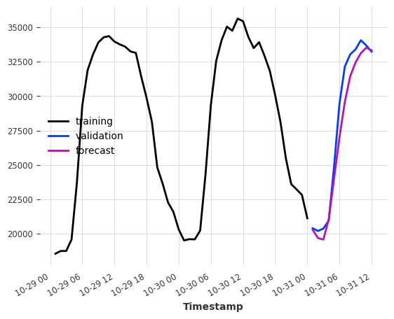
Let’s assume that instead of having weather measurements, we actually have weather forecasts. Then we could use them as future_covariates. We only do this here for demonstration purposes!
Below is an example that uses the last 24 hours (24) from hour target series (electricity consumption) and the values at the predicted time step ([0]) of our weather “forecasts”.
[5]:
model = LinearRegressionModel(lags=24, lags_future_covariates=[0])
model.fit(ts_energy_train, future_covariates=ts_weather)
pred = model.predict(12)

ts_energy_train[-48:].plot(label="training")
ts_energy_val[:12].plot(label="validation")
pred.plot(label="forecast")
[5]:
<Axes: xlabel='Timestamp'>
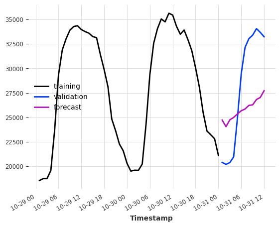
Using only covariates
Sometimes, we might also be interested in a forecasting model that purely relies on the covariates values.
To do this, specify at least one of lags_past_covariates or lags_future_covariates and set lags=None. Darts regression models are trained in a supervised manner, so we still have to provide the target series for training.
How well can we predict the electricity consumption using only the weather “forecasts” as input?
The lags tuple (24, 1) means (number of lags in the past, number of lags in the future).
[6]:
model = LinearRegressionModel(lags=None, lags_future_covariates=(24, 1))
model.fit(series=ts_energy_train, future_covariates=ts_weather)
pred = model.predict(12)

ts_energy_train[-48:].plot(label="training")
ts_energy_val[:12].plot(label="validation")
pred.plot(label="forecast")
[6]:
<Axes: xlabel='Timestamp'>
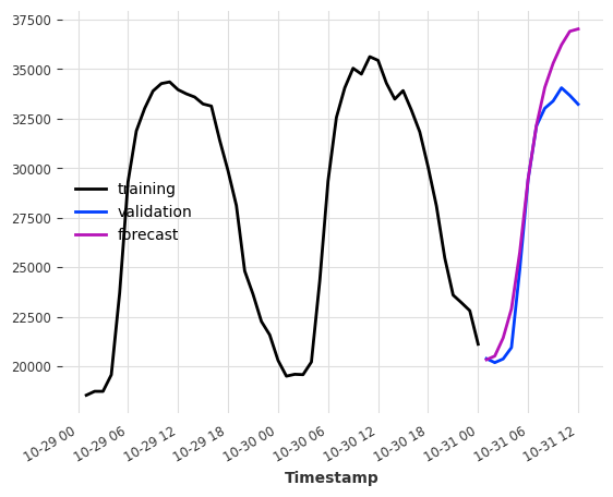
And what if we added some calendar information? We can let the model generate calendar attribute encodings for free with add_encoders.
[7]:
model = LinearRegressionModel(
    lags=None,
    lags_future_covariates=(24, 1),
    add_encoders={
        "cyclic": {"future": ["minute", "hour", "dayofweek", "month"]},
        "tz": "CET",
    },
)
model.fit(series=ts_energy_train, future_covariates=ts_weather)
pred = model.predict(12)

ts_energy_train[-48:].plot(label="training")
ts_energy_val[:12].plot(label="validation")
pred.plot(label="forecast")
plt.show()
Component-specific lags
If the target or any of the covariates is multivariate (has multiple components/columns), we can use dedicated lags for each component. Just pass a dictionary to the lags* parameters with the component name as key and the lags as value.
In the example below, we set the default lags to (24,1) (used for the covariates components 'T [°C]' and 'StrGlo [W/ms]') and give feature 'RainDur [min]' a dedicated lag [0].
[8]:
model = LinearRegressionModel(
    lags=None, lags_future_covariates={"default_lags": (24, 1), "RainDur [min]": [0]}
)
model.fit(series=ts_energy_train, future_covariates=ts_weather)
pred = model.predict(12)

ts_energy_train[-48:].plot(label="training data")
ts_energy_val[:12].plot(label="validation data")
pred.plot(label="forecast")
[8]:
<Axes: xlabel='Timestamp'>
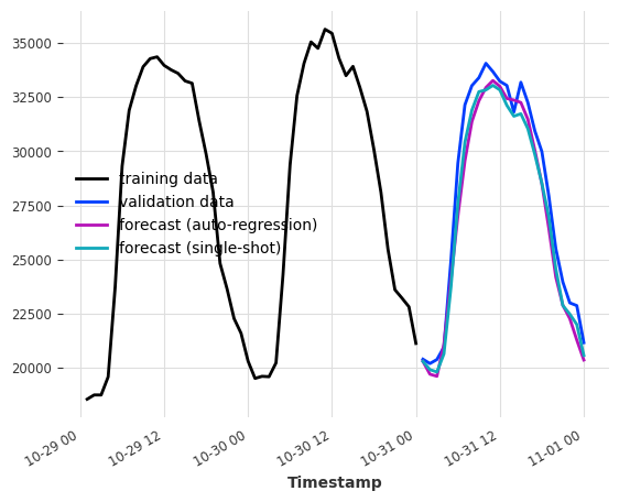
Model’s output chunk length
This key parameter sets the number of time steps that can be predicted at once by the internal regression model.
It is not the same as forecast horizon n from predict() which is the desired the number of generated prediction points, that is achieved either with: - a single shot forecast (if n <= output_chunk_length), or - an auto-regressive forecast, consuming its own forecast (and future values of covariates) as input for additional predictions (otherwise)
For example, if we want our model to forecast the next 24 hours of electricity consumption based on the last day of consumption, setting output_chunk_length=24 ensures that the model will not consume its forecasts or future values of our covariates to predict the entire day.
[9]:
model_auto_regression = LinearRegressionModel(lags=24, output_chunk_length=1)
model_single_shot = LinearRegressionModel(lags=24, output_chunk_length=24)

model_auto_regression.fit(ts_energy_train)
model_single_shot.fit(ts_energy_train)

pred_auto_regression = model_auto_regression.predict(24)
pred_single_shot = model_single_shot.predict(24)

ts_energy_train[-48:].plot(label="training data")
ts_energy_val[:24].plot(label="validation data")
pred_auto_regression.plot(label="forecast (auto-regression)")
pred_single_shot.plot(label="forecast (single-shot)")
[9]:
<Axes: xlabel='Timestamp'>
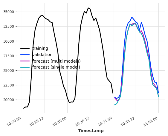
Multi-model forecasting
When output_chunk_length>1, the model behavior can be further parametrized by modifying the multi_models argument.
multi_models=True is the default behavior in Darts and was shown above. We create output_chunk_length copies of the model, and train each of them to predict one of the output_chunk_length time steps (using the same inputs). This approach is more computationally and memory intensive but tends to yield better results.
Single-model forecasting
When multi_model=False, we use a single model and train it to predict only the last point in output_chunk_length. This reduces model complexity as only a single set of coefficients will be trained and stored.
We are still able to predict all points from 1 until output_chunk_length by shifting the lags during tabularization. This means that a new set of input values is used for each forecasted value. Due to the shifting, the minimum length requirement for the training series will also be increased.
[10]:
multi_models = LinearRegressionModel(lags=24, output_chunk_length=24, multi_models=True)
single_model = LinearRegressionModel(
    lags=24, output_chunk_length=24, multi_models=False
)

multi_models.fit(ts_energy_train)
single_model.fit(ts_energy_train)

pred_multi_models = multi_models.predict(24)
pred_single_model = single_model.predict(24)

ts_energy_train[-48:].plot(label="training")
ts_energy_val[:24].plot(label="validation")
pred_multi_models.plot(label="forecast (multi models)")
pred_single_model.plot(label="forecast (single model)")
[10]:
<Axes: xlabel='Timestamp'>
Visualization
To vizualize what is happening under the hood, let’s simplify the model a bit and show the process for different parameters.
Model setup: LinearRegressionModel(lags=[-4, -3, -2, -1], output_chunk_length=2, multi_models=True).
When calling predict(n=4), the input series is processed as follows:
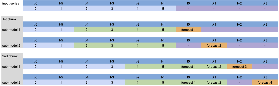
Since n>output_chunk_length, the model had to use auto-regression and the forecasted period is composed of two chunks of size output_chunk_length. There was no lags shift per output chunk because multi_models=True.
Model setup: LinearRegressionModel(lags=[-4, -3, -2, -1], output_chunk_length=2, multi_models=False).
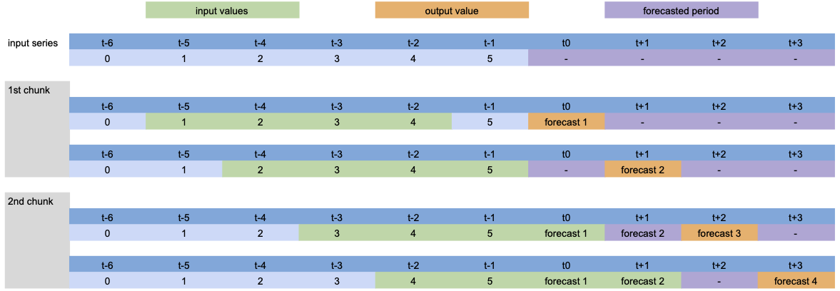
Apart from the auto-regressive prediction, we can see the lags shift per predicted time step because multi_models=False.
The same process also occurs during tabularizion for training the model: each green chunk is paired with an orange value, constituting the training dataset.
Probabilistic forecasting
To make a model probablistic, set parameter likelihood to quantile or poisson when creating a RegressionModel. At prediction time, probabilistic models can either : - use Monte Carlo sampling to generate samples based on the fitted distribution parameters when num_samples > 1 - return the fitted distribution parameters when predict_likelihood_parameters=True
Note that when using the quantile regressor, each quantile will be fitted by a different model.
Probabilistic models will generate different forecasts each time predict() is called with num_samples > 1. To get reproducible results, set the random seed when creating the model and call the methods in the exact same order.
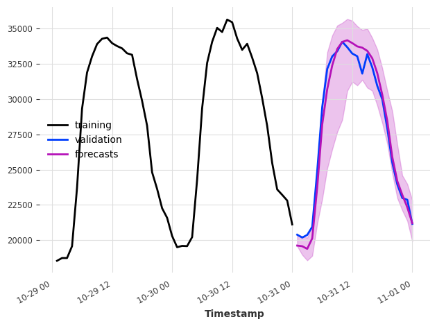
[11]:
model = XGBModel(
    lags=24, output_chunk_length=1, likelihood="quantile", quantiles=[0.05, 0.5, 0.95]
)

model.fit(ts_energy_train)

pred_samples = model.predict(n=24, num_samples=200)
pred_params = model.predict(n=1, num_samples=1, predict_likelihood_parameters=True)

for val, comp in zip(pred_params.values()[0], pred_params.components):
    print(f"{comp} : {round(val, 3)}")

ts_energy_train[-48:].plot(label="training")
ts_energy_val[:24].plot(label="validation")
pred_samples.plot(label="forecasts")
plt.tight_layout()
Value_NE5_q0.05 : 19580.123046875
Value_NE5_q0.50 : 19623.302734375
Value_NE5_q0.95 : 20418.7421875
MultiOutputRegressor wrapper
Some regression models support native multi-output support. This is required to fit and predict: - multiple outputs/multiple target steps (with output_chunk_length>1 and multi_models=True) - probabilistic models using quantile regression - multivariates series
For models that don’t support it, Darts wraps sklearn’s MultiOutputRegressor around them to handle the logic under the hood.
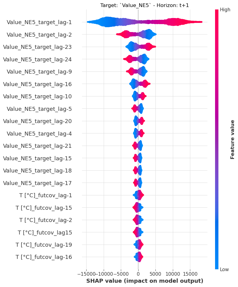
Explainability
We offer explainability for the regression models with Darts’ ShapExplainer. The explainer uses shap, a library based on game theory, to give insights into feature importances over time for our forecast horizon.
[12]:
model = LinearRegressionModel(lags=24, lags_future_covariates=(24, 24))
model.fit(ts_energy_train, future_covariates=ts_weather)
shap_explainer = ShapExplainer(model=model)
shap_values = shap_explainer.summary_plot()
No data for colormapping provided via 'c'. Parameters 'vmin', 'vmax' will be ignored
[13]:
# extracting the end of each series to reduce computation time
foreground_target = ts_energy_train[-24 * 2 :]
foreground_future_cov = ts_weather[foreground_target.start_time() :]

shap_explainer.force_plot_from_ts(
    foreground_series=foreground_target,
    foreground_future_covariates=foreground_future_cov,
)

# the plot cannot be rendered on GitHub or the Documentation page. Run it locally to see it.
[13]:
Have you run `initjs()` in this notebook? If this notebook was from another user you must also trust this notebook (File -> Trust notebook). If you are viewing this notebook on github the Javascript has been stripped for security. If you are using JupyterLab this error is because a JupyterLab extension has not yet been written.
Conclusion
By tabularizing the data and unifying the API across libraries, Darts closes the gap between traditional regression problems and timeseries forecasting.
RegressionModel and its sub-classes offer a wide range of functionalities which can be used to build strong models in just a few lines of codes.
Appendix
RegressionModel
RegressionModel wraps the Darts API around any sklearn regression model. With this we can use the model in the same way as any other Darts forecasting models.
As an examnple, fitting a Bayesian ridge regression on the example dataset takes only a few lines:
[14]:
model = RegressionModel(
    lags=24,
    lags_future_covariates=(48, 24),
    model=BayesianRidge(),
    output_chunk_length=24,
)

model.fit(ts_energy_train, future_covariates=ts_weather)

pred = model.predict(n=24)

ts_energy_train[-48:].plot(label="training")
ts_energy_val[:24].plot(label="validation")
pred.plot(label="forecast")
[14]:
<Axes: xlabel='Timestamp'>
The underlying model methods remain accessible and by combining the BasesianRidge.coef_ attribute with the RegressionModel.lagged_feature_names attribute, the coefficients of the regression model can easily be interpreted:
[15]:
# extract the coefficients of the first timestemp estimator
coef_values = model.model.estimators_[0].coef_
# get the lagged features name
coef_names = model.lagged_feature_names
# combine them in a dict
coefficients = {name: val for name, val in zip(coef_names, coef_values)}
# see the coefficient of the target value at last timestep before the forecasted period
{c_name: c_val for idx, (c_name, c_val) in enumerate(coefficients.items()) if idx < 5}
[15]:
{'Value_NE5_target_lag-24': -0.3195560563281926,
 'Value_NE5_target_lag-23': 0.37621876784175745,
 'Value_NE5_target_lag-22': 0.005325414282057739,
 'Value_NE5_target_lag-21': -0.11885377506043901,
 'Value_NE5_target_lag-20': 0.12892167797527437}
One of the limitation of the RegressionModel class is that it does not provide probabilistic forecasting out of the box but it is possible to implement it by creating a new class inheriting from both RegressionModel and _LikelihoodMixin and implementing the missing methods (the LinearRegressionModel class can be use as a template).
Custom model
You can even implement your own model as long as it works with tabular data and provides the fit() and predict() methods:
[16]:
class CustomRegressionModel:
    def __init__(self, weights: np.ndarray):
        """Barebone weighted average"""
        self.weights = weights
        self.norm_coef = sum(weights)

    def fit(self, X: np.ndarray, y: np.ndarray, *args, **kwargs):
        return self

    def predict(self, X: np.ndarray):
        """Apply weights on each sample"""
        return (
            np.stack([np.correlate(x, self.weights, mode="valid") for x in X])
            / self.norm_coef
        )

    def get_params(self, deep: bool):
        return {"weights": self.weights}


window_weights = np.arange(1, 25, 1) ** 2
model = RegressionModel(
    lags=24,
    output_chunk_length=24,
    model=CustomRegressionModel(window_weights),
    multi_models=False,
)
model.fit(ts_energy_train)
pred = model.predict(n=24)

ts_energy_train[-48:].plot(label="training")
ts_energy_val[:24].plot(label="validation")
pred.plot(label="forecast")
[16]:
<Axes: xlabel='Timestamp'>
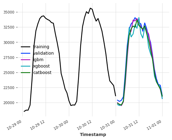
Example of the boosted tree models
Make sure to have the dependencies for lightgbm and catboost installed. You can check out our installation guide here
[17]:
lgbm_model = LightGBMModel(lags=24, output_chunk_length=24, verbose=0)
xgboost_model = XGBModel(lags=24, output_chunk_length=24)
catboost_model = CatBoostModel(lags=24, output_chunk_length=24)

lgbm_model.fit(ts_energy_train)
xgboost_model.fit(ts_energy_train)
catboost_model.fit(ts_energy_train)

pred_lgbm = lgbm_model.predict(n=24)
pred_xgboost = xgboost_model.predict(n=24)
pred_catboost = catboost_model.predict(n=24)

print(f"LightGBMModel MAPE: {mape(ts_energy_val, pred_lgbm)}")
print(f"XGBoostModel MAPE: {mape(ts_energy_val, pred_xgboost)}")
print(f"CatboostModel MAPE: {mape(ts_energy_val, pred_catboost)}")

ts_energy_train[-48:].plot(label="training")
ts_energy_val[:24].plot(label="validation")
pred_lgbm.plot(label="lgbm")
pred_xgboost.plot(label="xgboost")
pred_catboost.plot(label="catboost")
LightGBMModel MAPE: 2.2682070257112743
XGBoostModel MAPE: 3.5364068635935895
CatboostModel MAPE: 2.373275454432286
[17]:
<Axes: xlabel='Timestamp'>