Multiple Time Series, Pre-trained Models and Covariates

This notebook serves as a tutorial for:

• Training a single model on multiple time series

• Using a pre-trained model to obtain forecasts for any time series unseen during training

• Training and using a model using covariates

• Training and using a model using one or several multivariates TimeSeries

First, some necessary imports:

# fix python path if working locally
from utils import fix_pythonpath_if_working_locally

fix_pythonpath_if_working_locally()

import pandas as pd
import numpy as np
import torch
import matplotlib.pyplot as plt

from darts import TimeSeries, concatenate
from darts.utils.callbacks import TFMProgressBar
from darts.utils.timeseries_generation import (
    gaussian_timeseries,
    linear_timeseries,
    sine_timeseries,
)
from darts.models import (
    RNNModel,
    TCNModel,
    TransformerModel,
    NBEATSModel,
    BlockRNNModel,
    VARIMA,
)
from darts.metrics import mape, smape, mae
from darts.dataprocessing.transformers import Scaler
from darts.utils.timeseries_generation import datetime_attribute_timeseries
from darts.datasets import AirPassengersDataset, MonthlyMilkDataset, ElectricityDataset

import logging

logging.disable(logging.CRITICAL)

import warnings

warnings.filterwarnings("ignore")

%matplotlib inline

# for reproducibility
torch.manual_seed(1)
np.random.seed(1)


def generate_torch_kwargs():
    # run torch models on CPU, and disable progress bars for all model stages except training.
    return {
        "pl_trainer_kwargs": {
            "accelerator": "cpu",
            "callbacks": [TFMProgressBar(enable_train_bar_only=True)],
        }
    }

Read Data

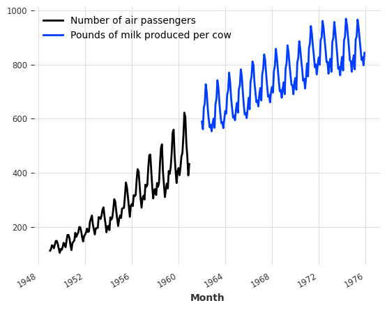
Let’s start by reading two time series - one containing the monthly number of air passengers, and another containing the monthly milk production per cow. These time series have not much to do with each other, except that they both have a monthly frequency with a marked yearly periodicity and upward trend, and (completely coincidentaly) they contain values of a comparable order of magnitude.

series_air = AirPassengersDataset().load()
series_milk = MonthlyMilkDataset().load()

series_air.plot(label="Number of air passengers")
series_milk.plot(label="Pounds of milk produced per cow")
plt.legend();

Preprocessing

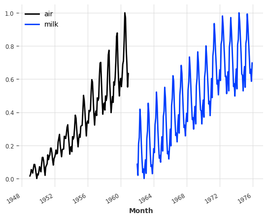
Usually neural networks tend to work better on normalised/standardised data. Here we’ll use the Scaler class to normalise both of our time series between 0 and 1:

scaler_air, scaler_milk = Scaler(), Scaler()
series_air_scaled = scaler_air.fit_transform(series_air)
series_milk_scaled = scaler_milk.fit_transform(series_milk)

series_air_scaled.plot(label="air")
series_milk_scaled.plot(label="milk")
plt.legend();

Train / Validation split

Let’s keep the last 36 months of both series as validation:

train_air, val_air = series_air_scaled[:-36], series_air_scaled[-36:]
train_milk, val_milk = series_milk_scaled[:-36], series_milk_scaled[-36:]

Global Forecasting Models

Darts contains many forecasting models, but not all of them can be trained on several time series. The models that support training on multiple series are called global models. An exhaustive list of the global models can be found here (bottom of the table) with for example:

• LinearRegressionModel

• BlockRNNModel

• Temporal Convolutional Networks (TCNModel)

• N-Beats (NBEATSModel)

• TiDEModel

In the following, we will distinguish two sorts of time series:

• The target time series is the time series we are interested to forecast (given its history)

• A covariate time series is a time series which may help in the forecasting of the target series, but that we are not interested in forecasting. It’s sometimes also called external data.

Note: Static covariates are invariant in time and correspond to additional information associated with the components of the target time series. Detailed information about this kind of covariate can be found in the static covariates notebook.

We further differentiate covariates series, depending on whether they can be known in advance or not:

• Past Covariates denote time series whose past values are known at prediction time. These are usually things that have to be measured or observed.

• Future Covariates denote time series whose future values are already known at prediction time for the span of the forecast horizon. These can for instance represent known future holidays, or weather forecasts.

Some models use only past covariates, others use only future covariates, and some models might use both. We will dive deeper in this topic in some other notebook, but this table details the covariates supported by each model.

All of the global models listed above support training on multiple series. In addition, they also all support multivariate series. This means that they can seamlessly be used with time series of more than one dimension; the target series can contain one (as is often the case) or several dimensions. A time series with several dimensions is really just a regular time series where the values at each time stamps are vectors instead of scalars.

As an example, the BlockRNNModel, N-Beats, TCN and Transformer models follow a “block” architecture. They contain a neural network that takes chunks of time series in input, and outputs chunks of (predicted) future time series values. The input dimensionality is the number of dimensions (components) of the target series, plus the number of components of all the covariates - stacked together. The output dimensionality is simply the number of dimensions of the target series: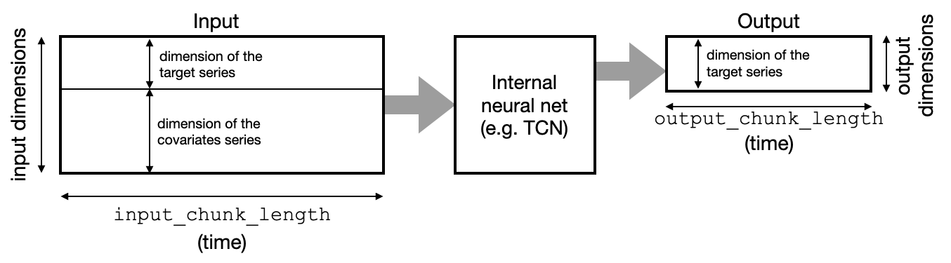

The RNNModel works differently, in a recurrent fashion (which is also why they support future covariates). The good news is that as a user, we don’t have to worry too much about the different model types and input/output dimensionalities. The dimensionalities are automatically inferred for us by the model based on the training data, and the support for past or future covariates is simply handled by the past_covariates or future_covariates arguments.

We’ll still have to specify two important parameters when building our models:

• input_chunk_length: this is the length of the lookback window of the model; so each output will be computed by the model by reading the previous input_chunk_length points.

• output_chunk_length: this is the length of the outputs (forecasts) produced by the internal model. However, the predict() method of the “outer” Darts model (e.g., the one of NBEATSModel, TCNModel, etc) can be called for a longer time horizon. In these cases, if predict() is called for a horizon longer than output_chunk_length, the internal model will simply be called repeatedly, feeding on its own previous outputs in an auto-regressive fashion. If past_covariates are used it requires these covariates to be known for long enough in advance.

Example with one Series

Let’s look at a first example. We’ll build an N-BEATS model that has a lookback window of 24 points (input_chunk_length=24) and predicts the next 12 points (output_chunk_length=12). We chose these values so it’ll make our model produce successive predictions for one year at a time, looking at the past two years.

model_air = NBEATSModel(
    input_chunk_length=24,
    output_chunk_length=12,
    n_epochs=200,
    random_state=0,
    **generate_torch_kwargs()
)

This model can be used like any other Darts forecasting model, beeing fit on a single time series:

model_air.fit(train_air)

NBEATSModel(generic_architecture=True, num_stacks=30, num_blocks=1, num_layers=4, layer_widths=256, expansion_coefficient_dim=5, trend_polynomial_degree=2, dropout=0.0, activation=ReLU, input_chunk_length=24, output_chunk_length=12, n_epochs=200, random_state=0, pl_trainer_kwargs={'accelerator': 'cpu', 'callbacks': [<darts.utils.callbacks.TFMProgressBar object at 0x103d1a710>]})

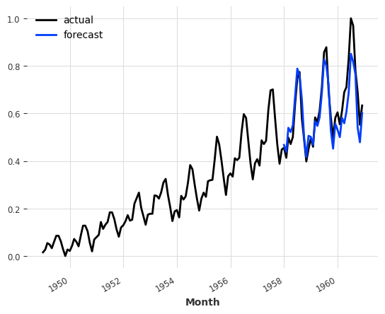
And like any other Darts forecasting models, we can then get a forecast by calling predict(). Note that below, we are calling predict() with a horizon of 36, which is longer than the model internal output_chunk_length of 12. That’s not a problem here - as explained above, in such a case the internal model will simply be called auto-regressively on its own outputs. In this case, it will be called three times so that the three 12-points outputs make up the final 36-points forecast - but all of this is done transparently behind the scenes.

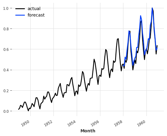
pred = model_air.predict(n=36)

series_air_scaled.plot(label="actual")
pred.plot(label="forecast")
plt.legend()
print("MAPE = {:.2f}%".format(mape(series_air_scaled, pred)))

MAPE = 8.02%

Training Process (behind the scenes)

So what happened when we called model_air.fit() above?

In order to train the internal neural network, Darts first makes a dataset of inputs/outputs examples from the provided time series (in this case: series_air_scaled). There are several ways this can be done and Darts contains a few different dataset implementations in the darts.utils.data package.

By default, NBEATSModel will instantiate a darts.utils.data.PastCovariatesSequentialDataset, which simply builds all the consecutive pairs of input/output sub-sequences (of lengths input_chunk_length and output_chunk_length) existing in the series).

For an example series of length 14, with input_chunk_length=4 and output_chunk_length=2, it looks as follows: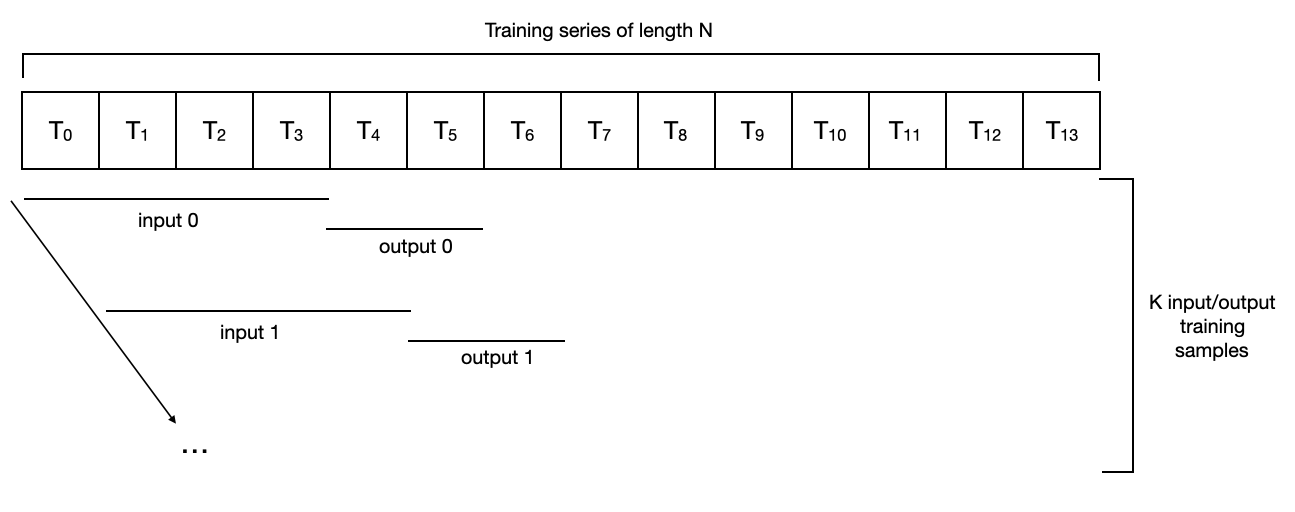

For such a dataset, a series of length N would result in a “training set” of N - input_chunk_length - output_chunk_length + 1 samples. In the toy example above, we have N=14, input_chunk_length=4 and output_chunk_length=2, so the number of samples used for training would be K = 9. In this context, a training epoch consists in complete pass (possibly consisting of several mini-batches) over all the samples.

Note that different models are susceptible to use different datasets by default. For instance, darts.utils.data.HorizonBasedDataset is inspired by the N-BEATS paper and produces samples that are “close” to the end of the series, possibly even ignoring the beginning of the series.

If you have the need to control the way training samples are produced from TimeSeries instances, you can implement your own training dataset by inheriting the abstract darts.utils.data.TrainingDataset class. Darts datasets are inheriting from torch Dataset, which means it’s easy to implement lazy versions that do not load all data in memory at once. Once you have your own instance of a dataset, you can directly call the fit_from_dataset() method, which is supported by all global forecasting models.

Training a Model on Multiple Time Series

All this machinery can be seamlessly used with multiple time series. Here’s how a sequential dataset with input_chunk_length=4 and output_chunk_length=2 looks for two series of lengths N and M:

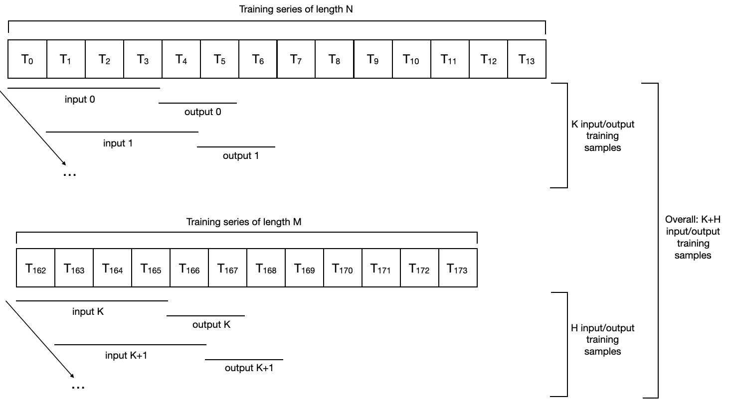
Note a few things here:

• The different series do not need to have the same length, or even to share the same time stamps.

• In fact, they don’t even need to have the same frequency.

• The total number of samples in the training dataset will be the union of all the training samples contained in each series; so a training epoch will now span all samples from all series.

Training on Both Air Traffic and Milk Series

Let’s look at another example where we fit another model instance on our two time series (air passengers and milk production). Since using two series of (roughly) the same length (roughly) doubles the training dataset size, we will use half of the number of epochs:

model_air_milk = NBEATSModel(
    input_chunk_length=24,
    output_chunk_length=12,
    n_epochs=100,
    random_state=0,
    **generate_torch_kwargs()
)

Then, fitting the model on two (or more) series is as simple as giving a list of series (instead of a single series) in argument to the fit() function:

model_air_milk.fit([train_air, train_milk])

NBEATSModel(generic_architecture=True, num_stacks=30, num_blocks=1, num_layers=4, layer_widths=256, expansion_coefficient_dim=5, trend_polynomial_degree=2, dropout=0.0, activation=ReLU, input_chunk_length=24, output_chunk_length=12, n_epochs=100, random_state=0, pl_trainer_kwargs={'accelerator': 'cpu', 'callbacks': [<darts.utils.callbacks.TFMProgressBar object at 0x2af748f10>]})

Producing Forecasts After the End of a Series

Now, importantly, when computing the forecasts we have to specify which time series we want to forecast the future for.

We didn’t have this constraint earlier. When fitting models on one series only, the model remembers this series internally, and if predict() is called without the series argument, it returns a forecast for the (unique) training series. This does not work anymore as soon as a model is fit on more than one series - in this case the series argument of predict() becomes mandatory.

So, let’s say we want to predict future of air traffic. In this case we specify series=train_air to the predict() function in order to say we want to get a forecast for what comes after train_air:

pred = model_air_milk.predict(n=36, series=train_air)

series_air_scaled.plot(label="actual")
pred.plot(label="forecast")
plt.legend()
print("MAPE = {:.2f}%".format(mape(series_air_scaled, pred)))

MAPE = 7.58%

Wait… does this mean that milk production helps to predict air traffic??

Well, in this particular instance with this model, it seems to be the case (at least in terms of MAPE error). This is not so weird if you think about it, though. Air traffic is heavily characterized by the yearly seasonality and upward trend. The milk series exhibits these two traits as well, and in this case it’s probably helping the model to capture them.

Note that this points towards the possibility of pre-training forecasting models; training models once and for all and later using them to forecast series that are not in the train set. With our toy model we can really forecast the future values of any other series, even series never seen during training. For the sake of example, let’s say we want to forecast the future of some arbitrary sine wave series:

any_series = sine_timeseries(length=50, freq="M")
pred = model_air_milk.predict(n=36, series=any_series)

any_series.plot(label='"any series, really"')
pred.plot(label="forecast")
plt.legend()

<matplotlib.legend.Legend at 0x2af20d5d0>

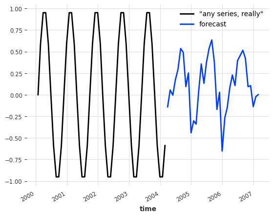
This forecast isn’t good (the sine doesn’t even have a yearly seasonality), but you get the idea.

Similar to what is supported by the fit() function, we can also give a list of series in argument to the predict() function, in which case it will return a list of forecast series. For example, we can get the forecasts for both the air traffic and the milk series in one go as follows:

pred_list = model_air_milk.predict(n=36, series=[train_air, train_milk])
for series, label in zip(pred_list, ["air passengers", "milk production"]):
    series.plot(label=f"forecast {label}")
plt.legend()

<matplotlib.legend.Legend at 0x2b56bb9d0>

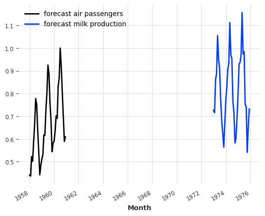
The two series returned correspond to the forecasts after the end of train_air and train_milk, respectively.

Covariates Series

Until now, we have only been playing with models that only use the history of the target series to predict its future. However, as explained above, the global Darts models also support the use of covariates time series. These are time series of “external data”, which we are not necessarily interested in predicting, but which we would still like to feed as input of our models because they can contain valuable information.

Building Covariates

Let’s see a simple example with our air and milk series, where we’ll try to use the year and month-of-the-year as covariates:

# build year and month series:
air_year = datetime_attribute_timeseries(series_air_scaled, attribute="year")
air_month = datetime_attribute_timeseries(series_air_scaled, attribute="month")

milk_year = datetime_attribute_timeseries(series_milk_scaled, attribute="year")
milk_month = datetime_attribute_timeseries(series_milk_scaled, attribute="month")

# stack year and month to obtain series of 2 dimensions (year and month):
air_covariates = air_year.stack(air_month)
milk_covariates = milk_year.stack(milk_month)

# split in train/validation sets:
air_train_covariates, air_val_covariates = air_covariates[:-36], air_covariates[-36:]
milk_train_covariates, milk_val_covariates = (
    milk_covariates[:-36],
    milk_covariates[-36:],
)

# scale them between 0 and 1:
scaler_covariates = Scaler()
air_train_covariates, milk_train_covariates = scaler_covariates.fit_transform(
    [air_train_covariates, milk_train_covariates]
)
air_val_covariates, milk_val_covariates = scaler_covariates.transform(
    [air_val_covariates, milk_val_covariates]
)

# concatenate for the full scaled series; we can feed this to model.fit()/predict() as Darts will extract the required covariates for you
air_covariates = concatenate([air_train_covariates, air_val_covariates])
milk_covariates = concatenate([milk_train_covariates, milk_val_covariates])

# plot the covariates:
plt.figure()
air_covariates.plot()
plt.title("Air traffic covariates (year and month)")

plt.figure()
milk_covariates.plot()
plt.title("Milk production covariates (year and month)")

Text(0.5, 1.0, 'Milk production covariates (year and month)')

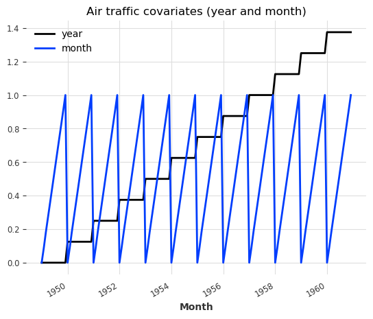
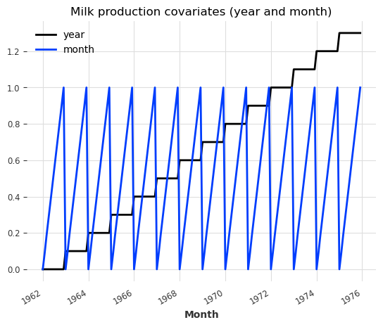
Good, so for each target series (air and milk), we have built a covariates series having the same time axis and containing the year and the month.

Note that here the covariates series are multivariate time series: they contain two dimensions - one dimension for the year and one for the month.

Training with Covariates

Let’s revisit our example again, this time with covariates. We will build a BlockRNNModel here. We activate checkpointing to keep track of the model performance on a validation set over time.

model_name = "BlockRNN_test"
model_pastcov = BlockRNNModel(
    model="LSTM",
    input_chunk_length=24,
    output_chunk_length=12,
    n_epochs=100,
    random_state=0,
    model_name=model_name,
    save_checkpoints=True,  # store model states: latest and best performing of validation set
    force_reset=True,
    **generate_torch_kwargs()
)

Now, to train the model with covariates, it is as simple as providing the covariates (in form of a list matching the target series) as past_covariates argument to the fit() function. The argument is named past_covariates to remind us that the model can use past values of these covariates in order to make a prediction. We can feed the entire air and milk covariates including the train and test sets to model.fit()/predict() as Darts will automatically extract the required covariates for you.

Aditionally, we pass a validation series to avoid model overfitting.

model_pastcov.fit(
    series=[train_air, train_milk],
    past_covariates=[air_covariates, milk_covariates],
    val_series=[val_air, val_milk],
    val_past_covariates=[air_covariates, milk_covariates],
)

BlockRNNModel(model=LSTM, hidden_dim=25, n_rnn_layers=1, hidden_fc_sizes=None, dropout=0.0, input_chunk_length=24, output_chunk_length=12, n_epochs=100, random_state=0, model_name=BlockRNN_test, save_checkpoints=True, force_reset=True, pl_trainer_kwargs={'accelerator': 'cpu', 'callbacks': [<darts.utils.callbacks.TFMProgressBar object at 0x2b56bb640>]})

Now we load the model state with the best performance on the validation set to avoid overfitting.

model_pastcov = BlockRNNModel.load_from_checkpoint(model_name=model_name, best=True)

Since the covariates can easily be known in the future in this example, we can also define a RNNModel and train it using them as future_covariate:

model_name = "RNN_test"
model_futcov = RNNModel(
    model="LSTM",
    hidden_dim=20,
    batch_size=8,
    n_epochs=100,
    random_state=0,
    training_length=35,
    input_chunk_length=24,
    model_name=model_name,
    save_checkpoints=True,  # store model states: latest and best performing of validation set
    force_reset=True,
    **generate_torch_kwargs()
)

model_futcov.fit(
    series=[train_air, train_milk],
    future_covariates=[air_covariates, milk_covariates],
    val_series=[val_air, val_milk],
    val_future_covariates=[air_covariates, milk_covariates],
)

RNNModel(model=LSTM, hidden_dim=20, n_rnn_layers=1, dropout=0.0, training_length=35, batch_size=8, n_epochs=100, random_state=0, input_chunk_length=24, model_name=RNN_test, save_checkpoints=True, force_reset=True, pl_trainer_kwargs={'accelerator': 'cpu', 'callbacks': [<darts.utils.callbacks.TFMProgressBar object at 0x2b69cb9d0>]})

Now we load the model state with the best performance on the validation set to avoid overfitting.

model_futurecov = RNNModel.load_from_checkpoint(model_name=model_name, best=True)

Forecasting with Covariates

similarly, getting a forecast is now only a matter of specifying the past_covariates argument to the predict() function for the BlockRNNModel:

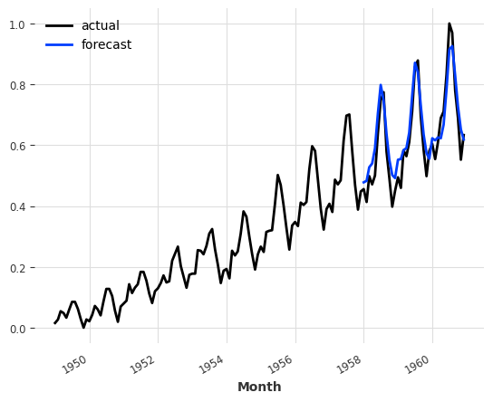
pred_cov = model_pastcov.predict(n=36, series=train_air, past_covariates=air_covariates)

series_air_scaled.plot(label="actual")
pred_cov.plot(label="forecast")
plt.legend()

<matplotlib.legend.Legend at 0x2b6abd4b0>

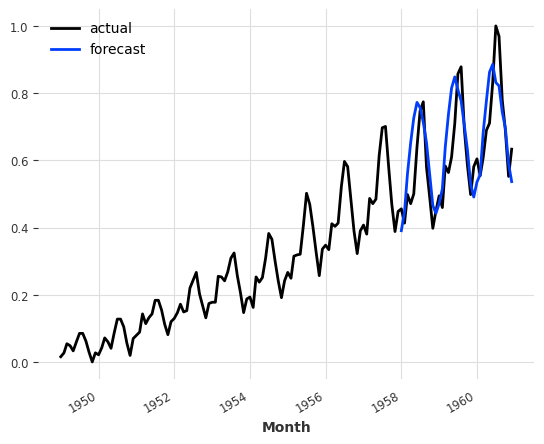
Note that here we called predict() with a forecast horizon n that is larger than the output_chunk_length we trained our model with. We were able to do this because even though BlockRNNModel uses past covariates, in this case these covariates are also known into the future, so Darts is able to compute the forecasts auto-regressively for n time steps in the future.

For the RNNModel, we can use a similar approach by just providing future_covariates to the predict() function:

pred_cov = model_futcov.predict(
    n=36, series=train_air, future_covariates=air_covariates
)

series_air_scaled.plot(label="actual")
pred_cov.plot(label="forecast")
plt.legend()

<matplotlib.legend.Legend at 0x2b6ba5540>

Backtesting with Covariates

We can also backtest the models using covariates. Say for instance we are interested in evaluating the running accuracy with a horizon of 12 months start at the beginning of the validation series.

• we start at the beginning of the validation series (start=val_air.start_time()).

• each prediction will have length forecast_horizon=12.

• the next prediction will start stride=12 points after the previous one

• we keep all predicted values from each forecast (last_points_only=False)

• the we continue until we run out of input data

In the end we concatenate the historical forecasts to get a single continuous (on time axis) time series

backtest_pastcov = model_pastcov.historical_forecasts(
    series_air_scaled,
    past_covariates=air_covariates,
    start=val_air.start_time(),
    forecast_horizon=12,
    stride=12,
    last_points_only=False,
    retrain=False,
    verbose=True,
)
backtest_pastcov = concatenate(backtest_pastcov)
print(
    "MAPE (BlockRNNModel with past covariates) = {:.2f}%".format(
        mape(series_air_scaled, backtest_pastcov)
    )
)

backtest_futcov = model_futcov.historical_forecasts(
    series_air_scaled,
    future_covariates=air_covariates,
    start=val_air.start_time(),
    forecast_horizon=12,
    stride=12,
    last_points_only=False,
    retrain=False,
    verbose=True,
)
backtest_futcov = concatenate(backtest_futcov)
print(
    "MAPE (RNNModel with future covariates) = {:.2f}%".format(
        mape(series_air_scaled, backtest_futcov)
    )
)

MAPE (BlockRNNModel with past covariates) = 12.09%

MAPE (RNNModel with future covariates) = 10.26%

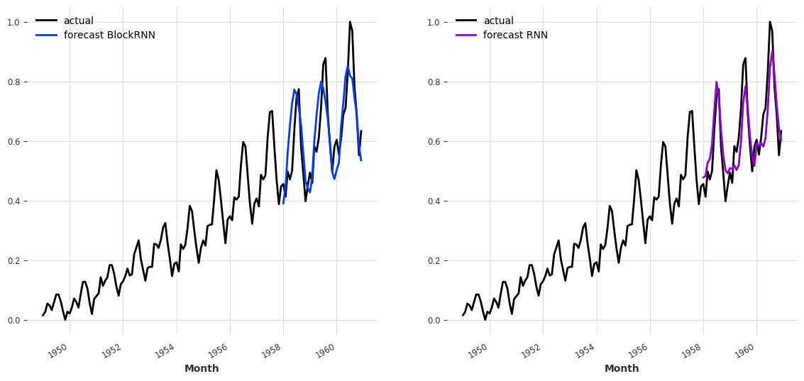
With the selected hyperparameters (and random seed), the BlockRNNModel using the past_covariates (MAPE=10.48%) seems to outperform the RNNModel with future_covariates (MAPE=15.21%). In order to have a better idea of the forecast obtained with these two models, it’s possible to plot them next to each other:

fig, axs = plt.subplots(1, 2, figsize=(14, 6))
series_air_scaled.plot(label="actual", ax=axs[0])
backtest_pastcov.plot(label="forecast BlockRNN", ax=axs[0])
axs[0].legend()
series_air_scaled.plot(label="actual", ax=axs[1])
backtest_futcov.plot(label="forecast RNN", ax=axs[1], color="darkviolet")
axs[1].legend()
plt.show()

A few more words on past covariates, future covariates and other conditioning

At the moment Darts supports covariates that are themselves time series. These covariates are used as model inputs, but are never themselves subject to prediction. The covariates do not necessarily have to be aligned with the target series (e.g. they do not need to start at the same time). Darts will use the actual time values of the TimeSeries time axes in order to jointly slice the targets and covariates correctly, both for training and inference. Of course the covariates still need to have a sufficient span, otherwise Darts will complain.

As explained above, TCNModel, NBEATSModel, BlockRNNModel, TransformerModel use past covariates (they will complain if you try using future_covariates). If these past covariates happen to also be known into the future, then these models are also able to produce forecasts for n > output_chunk_length (as shown above for BlockRNNModel) in an auto-regressive way.

By contrast, RNNModel uses future covariates (it will complain if you try specifying past_covariates). This means that prediction with this model requires the covariates (at least) n time steps into the future after prediction time.

Past and future covariates (as well as the way they are consumed by the different models) are an important but non-trivial topic, and we plan to dedicate a future notebook (or article) to explain this further.

Training and Forecasting Multivariate TimeSeries

Now, instead of having to forecast only one variable, we would like to forecast several of them at once. In constrast of the multi-series training, where two different univariate datasets were used to train a single model, the training set consists in a single serie containing observations for several variables (called components). These components usually present the same nature (measurement of the same metric) but this is not necessarily the case.

Even if not be covered in this example, models can also be trained using several multivariate TimeSeries by providing a sequence of such series to the fit method (on the condition that the model supports multivatiate TimeSeries of course).

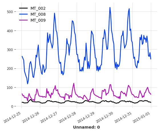
In order to illustrate this example, the ElectricityDataset (also available in Darts) will be used. This dataset contains measurements of electric power comsumption (in kW) for 370 clients with a sampling rate of 15 minutes.

multi_serie_elec = ElectricityDataset().load()

Since this multivariate serie is particularly large (370 components, 140’256 values), we keep only 3 components before resampling the serie with a frequency of 1 hour. Finally, the last 168 values (one week) are retained to shorten the training duration.

# retaining only three components in different ranges
retained_components = ["MT_002", "MT_008", "MT_009"]
multi_serie_elec = multi_serie_elec[retained_components]
# resampling the multivariate time serie
multi_serie_elec = multi_serie_elec.resample(freq="1H")
# keep the values for the last 5 days
multi_serie_elec = multi_serie_elec[-168:]

multi_serie_elec.plot()
plt.show()

Data preparation and inference routine

We split the dataset in training (6 days) and validation set (1 day) and normalize the values. In Darts, all the models are trained by calling fit and infer using predict, it is thus possible to define short function fit_and_pred to wrap these two steps.

# split in train/validation sets
training_set, validation_set = multi_serie_elec[:-24], multi_serie_elec[-24:]

# define a scaler, by default, normalize each component between 0 and 1
scaler_dataset = Scaler()
# scaler is fit on training set only to avoid leakage
training_scaled = scaler_dataset.fit_transform(training_set)
validation_scaled = scaler_dataset.transform(validation_set)


def fit_and_pred(model, training, validation):
    model.fit(training)
    forecast = model.predict(len(validation))
    return forecast

Now, we will define and train one VARIMA model and one RNNModel using the function defined above. Since the dataset is Integer-indexed, the trend argument for the VARIMA model must be set to None which is not really problematic since no trend is noticeable in the plot above.

model_VARIMA = VARIMA(p=12, d=0, q=0, trend="n")

model_GRU = RNNModel(
    input_chunk_length=24,
    model="LSTM",
    hidden_dim=25,
    n_rnn_layers=3,
    training_length=36,
    n_epochs=200,
    **generate_torch_kwargs()
)

# training and prediction with the VARIMA model
forecast_VARIMA = fit_and_pred(model_VARIMA, training_scaled, validation_scaled)
print("MAE (VARIMA) = {:.2f}".format(mae(validation_scaled, forecast_VARIMA)))

# training and prediction with the RNN model
forecast_RNN = fit_and_pred(model_GRU, training_scaled, validation_scaled)
print("MAE (RNN) = {:.2f}".format(mae(validation_scaled, forecast_RNN)))

MAE (VARIMA) = 0.11

MAE (RNN) = 0.10

Since we used a Scaler to normalize each component of the multivariate serie, we must not forget to scale them back in order to be able to properly visualise the forecasted values.

forecast_VARIMA = scaler_dataset.inverse_transform(forecast_VARIMA)
forecast_RNN = scaler_dataset.inverse_transform(forecast_RNN)

labels = [f"forecast {component}" for component in retained_components]
fig, axs = plt.subplots(1, 2, figsize=(14, 6))
validation_set.plot(ax=axs[0])
forecast_VARIMA.plot(label=labels, ax=axs[0])
axs[0].set_ylim(0, 500)
axs[0].set_title("VARIMA model forecast")
axs[0].legend(loc="upper left")
validation_set.plot(ax=axs[1])
forecast_RNN.plot(label=labels, ax=axs[1])
axs[1].set_ylim(0, 500)
axs[1].set_title("RNN model forecast")
axs[1].legend(loc="upper left")
plt.show()

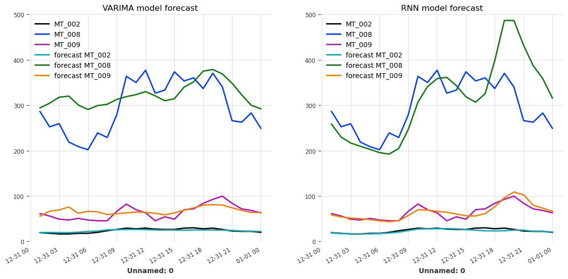
Due to the parameters selection, favoring speed over accuracy, the quality of the forecast is not great. Using more components from the original dataset or increasing the size of the training set should improve the accuracy of both models. Another possible improvement would be to account for the daily seasonality of the dataset by setting p (time lag) to 24 instead of 12 in the VARIMA model, and to retrain it.

Comments on training using multivariate series

All the features shown ealier on univariate TimeSeries, notably using covariates (past and future) or sequence of series, are of course also compatible with multivariate TimeSeries (just make sure that the model used actually supports them).

Furthermore, the models supporting multivariates series might use different approaches. TFTModel for example, uses a specialized module to select the relevant features whereas NBEATSModel flatten the serie’s components into an univariate serie and rely on its fully connected layers to capture the interactions between the features.

previous

Examples

next

Data (pre) processing using DataTransformer and Pipeline