Data (pre) processing using DataTransformer and Pipeline

In this notebook, we will demonstrate how to perform some common preprocessing tasks using darts

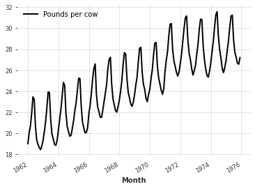
As a toy example, we will use the Monthly Milk Production dataset.

The DataTransformer abstraction

DataTransformer aims to provide a unified way of dealing with transformations of TimeSeries:

• transform() is implemented by all transformers. This method takes in either a TimeSeries of a sequence of TimeSeries, applies the transformation and returns it as a new TimeSeries/sequence of `TimeSeries.

• inverse_transform() is implemented by transformers for which an inverse transformation function exists. It works in a similar way as transform()

• fit() allows transformers to extract some information from the time series first before calling transform() or inverse_transform()

Setting up the example

# fix python path if working locally
from utils import fix_pythonpath_if_working_locally

fix_pythonpath_if_working_locally()

%load_ext autoreload
%autoreload 2
%matplotlib inline

import pandas as pd
import matplotlib.pyplot as plt
import numpy as np

from darts import TimeSeries
from darts.models import ExponentialSmoothing
from darts.dataprocessing.transformers import (
    Scaler,
    MissingValuesFiller,
    Mapper,
    InvertibleMapper,
)
from darts.dataprocessing import Pipeline
from darts.metrics import mape
from darts.utils.statistics import check_seasonality, plot_acf, plot_residuals_analysis
from darts.utils.timeseries_generation import linear_timeseries
from darts.datasets import MonthlyMilkDataset, MonthlyMilkIncompleteDataset

import warnings

warnings.filterwarnings("ignore")
import logging

logging.disable(logging.CRITICAL)

Reading the data and creating a time series

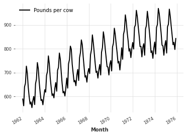
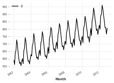
series = MonthlyMilkDataset().load()

print(series)
series.plot()

<TimeSeries (DataArray) (Month: 168, component: 1, sample: 1)>
array([[[589.]],

       [[561.]],

       [[640.]],

       [[656.]],

       [[727.]],

       [[697.]],

       [[640.]],

       [[599.]],

       [[568.]],

       [[577.]],

...

       [[892.]],

       [[903.]],

       [[966.]],

       [[937.]],

       [[896.]],

       [[858.]],

       [[817.]],

       [[827.]],

       [[797.]],

       [[843.]]])
Coordinates:
  * Month      (Month) datetime64[ns] 1962-01-01 1962-02-01 ... 1975-12-01
  * component  (component) object 'Pounds per cow'
Dimensions without coordinates: sample

Using a transformer: Rescaling a time series using Scaler.

Some applications may require your datapoints to be between 0 and 1 (e.g. to feed a time series to a Neural Network based forecasting model). This is easily achieved using the default Scaler, which is a wrapper around sklearn.preprocessing.MinMaxScaler(feature_range=(0, 1)).

scaler = Scaler()
rescaled = scaler.fit_transform(series)
print(rescaled)

<TimeSeries (DataArray) (Month: 168, component: 1, sample: 1)>
array([[[0.08653846]],

       [[0.01923077]],

       [[0.20913462]],

       [[0.24759615]],

       [[0.41826923]],

       [[0.34615385]],

       [[0.20913462]],

       [[0.11057692]],

       [[0.03605769]],

       [[0.05769231]],

...

       [[0.81490385]],

       [[0.84134615]],

       [[0.99278846]],

       [[0.92307692]],

       [[0.82451923]],

       [[0.73317308]],

       [[0.63461538]],

       [[0.65865385]],

       [[0.58653846]],

       [[0.69711538]]])
Coordinates:
  * Month      (Month) datetime64[ns] 1962-01-01 1962-02-01 ... 1975-12-01
  * component  (component) <U1 '0'
Dimensions without coordinates: sample

This scaling can easily be inverted too, by calling inverse_transform()

back = scaler.inverse_transform(rescaled)
print(back)

<TimeSeries (DataArray) (Month: 168, component: 1, sample: 1)>
array([[[589.]],

       [[561.]],

       [[640.]],

       [[656.]],

       [[727.]],

       [[697.]],

       [[640.]],

       [[599.]],

       [[568.]],

       [[577.]],

...

       [[892.]],

       [[903.]],

       [[966.]],

       [[937.]],

       [[896.]],

       [[858.]],

       [[817.]],

       [[827.]],

       [[797.]],

       [[843.]]])
Coordinates:
  * Month      (Month) datetime64[ns] 1962-01-01 1962-02-01 ... 1975-12-01
  * component  (component) <U1 '0'
Dimensions without coordinates: sample

Note that the Scaler also allows to specify other scalers in its constructor, as long as they implement fit(), transform() and inverse_transform() methods on TimeSeries (typically scalers from scikit-learn)

Another example : MissingValuesFiller

Let’s look at handling missing values in a dataset.

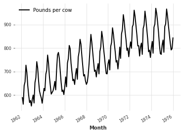
incomplete_series = MonthlyMilkIncompleteDataset().load()
incomplete_series.plot()

filler = MissingValuesFiller()
filled = filler.transform(incomplete_series, method="quadratic")

filled.plot()

Since MissingValuesFiller wraps around pd.interpolate by default, we can also provide arguments to the pd.interpolate() function when calling transform()

filled = filler.transform(incomplete_series, method="quadratic")
filled.plot()

Mapper and InvertibleMapper: A special kind of transformers

Sometimes you may want to perform a simple map() function on the data. This can also be done using data transformers. Mapper takes in a function and applies it to the data elementwise when calling transform().

InvertibleMapper also allows to specify an inverse function at creation (if there is one) and provides the inverse_transform() method.

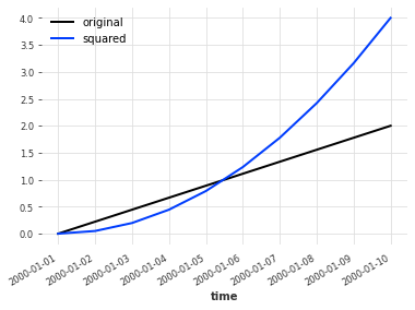
lin_series = linear_timeseries(start_value=0, end_value=2, length=10)

squarer = Mapper(lambda x: x**2)
squared = squarer.transform(lin_series)

lin_series.plot(label="original")
squared.plot(label="squared")
plt.legend()

<matplotlib.legend.Legend at 0x7ff5e3826c10>

More complex (and useful) transformations

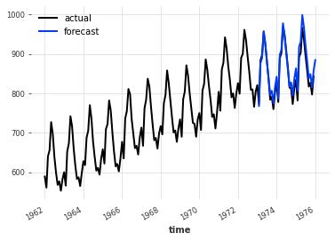
In the Monthly Milk Production dataset used earlier, some of the difference between the months comes from the fact that some months contain more days than others, resulting in a larger production of milk during those months. This makes the time series more complex, and thus harder to predict.

training, validation = series.split_before(pd.Timestamp("1973-01-01"))

model = ExponentialSmoothing()
model.fit(training)
forecast = model.predict(36)

plt.title("MAPE = {:.2f}%".format(mape(forecast, validation)))
series.plot(label="actual")
forecast.plot(label="forecast")
plt.legend()

<matplotlib.legend.Legend at 0x7ff5e3bcc790>

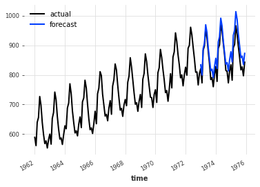
To take this fact into account and achieve better performance, we could instead:

1. Transform the time series to represent the average daily production of milk for each month (instead of the total production per month)

2. Make a forecast

3. Inverse the transformation

Let’s see how this would be implemented using InvertibleMapper and pd.timestamp.days_in_month

(Idea taken from “Forecasting: principles and Practice” by Hyndman and Athanasopoulos)

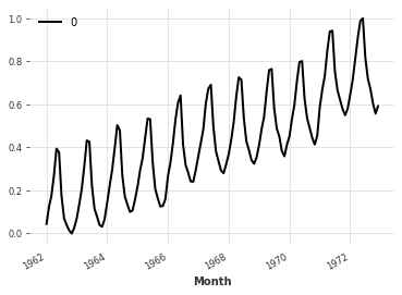
To transform the time series, we have to divide a monthly value (the data point) by the number of days in the month given by the value’s corresponding timestamp.

map() (and thus Mapper / InvertibleMapper) makes this convenient by allowing to apply a transformation function which uses both the value and its timestamp to compute the new value: f(timestamp, value) = new_value

# Transform the time series
toDailyAverage = InvertibleMapper(
    fn=lambda timestamp, x: x / timestamp.days_in_month,
    inverse_fn=lambda timestamp, x: x * timestamp.days_in_month,
)

dailyAverage = toDailyAverage.transform(series)

dailyAverage.plot()

# Make a forecast
dailyavg_train, dailyavg_val = dailyAverage.split_after(pd.Timestamp("1973-01-01"))

model = ExponentialSmoothing()
model.fit(dailyavg_train)
dailyavg_forecast = model.predict(36)

plt.title("MAPE = {:.2f}%".format(mape(dailyavg_forecast, dailyavg_val)))
dailyAverage.plot()
dailyavg_forecast.plot()
plt.legend()

<matplotlib.legend.Legend at 0x7ff5e3dd1ac0>

# Inverse the transformation
# Here the forecast is stochastic; so we take the median value
forecast = toDailyAverage.inverse_transform(dailyavg_forecast)

plt.title("MAPE = {:.2f}%".format(mape(forecast, validation)))
series.plot(label="actual")
forecast.plot(label="forecast")
plt.legend()

<matplotlib.legend.Legend at 0x7ff5e3fbb280>

Chaining transformations : introducing Pipeline

Now suppose that we both want to apply the above transformation (daily averaging), and rescale the dataset between 0 and 1 to use a Neural Network based forecasting model. Instead of applying these two transformations separately, and then inversing them separately, we can use a Pipeline.

pipeline = Pipeline([toDailyAverage, scaler])
transformed = pipeline.fit_transform(training)
transformed.plot()

If all transformations in the pipeline are invertible, the Pipeline object is too.

back = pipeline.inverse_transform(transformed)
back.plot()

Recall now the incomplete series from monthly-milk-incomplete.csv. Suppose that we want to encapsule all our preprocessing steps into a Pipeline, consisting of: a MissingValuesFiller for filling the missing values, and a Scaler for scaling the dataset between 0 and 1.

incomplete_series = MonthlyMilkIncompleteDataset().load()

filler = MissingValuesFiller()
scaler = Scaler()

pipeline = Pipeline([filler, scaler])
transformed = pipeline.fit_transform(incomplete_series)

Suppose we have trained a Neural Network and produced some predictions. Now, we want to scale back out data. Unfortunately, since the MissingValuesFiller is not an InvertibleDataTransformer (why on Earth would someone want to insert missing values in the results!?), the inverse transformation will raise an exception: ValueError: Not all transformers in the pipeline can perform inverse_transform.

Frustrating right? Fortunately, you don’t have to re-run everything from scratch, excluding the MissingValuesFiller from the Pipeline. Instead, you can just set the partial argument of the inverse_transform method to True. In this case, the inverse transformation will be performed skipping the not invertible transformers.

back = pipeline.inverse_transform(transformed, partial=True)

Processing multiple TimeSeries

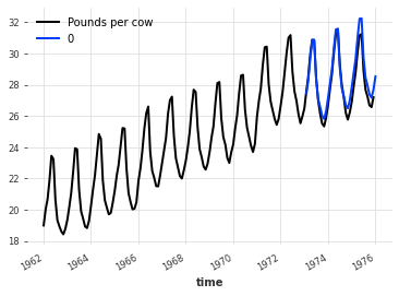
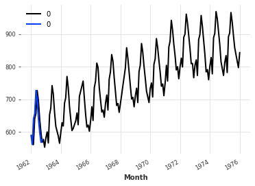
Often, we have to deal with multiple TimeSeries. DARTS supports Sequences of TimeSeries as input to transformers and pipelines, so that you don’t have to take care of processing each sample separately. Furthermore, it will take care of storing the parameters used by each scaler while transforming different TimeSeries (e.g., with scalers).

series = MonthlyMilkDataset().load()
incomplete_series = MonthlyMilkIncompleteDataset().load()

multiple_ts = [incomplete_series, series[:10]]

filler = MissingValuesFiller()
scaler = Scaler()

pipeline = Pipeline([filler, scaler])
transformed = pipeline.fit_transform(multiple_ts)

for ts in transformed:
    ts.plot()

back = pipeline.inverse_transform(transformed, partial=True)
for ts in back:
    ts.plot()

Monitoring & parallelising data processing

Sometimes, we could also have to deal with huge datasets. In this cases, processing each sample sequentially can take quite a long time. Darts can help both monitoring the transformations, and processing multiple samples in parallel, when possible.

Setting the verbose parameter in each transformer or pipeline while create some progress bars:

series = MonthlyMilkIncompleteDataset().load()

huge_number_of_series = [series] * 10000

scaler = Scaler(verbose=True, name="Basic")

transformed = scaler.fit_transform(huge_number_of_series)

We now know for how long we will have to wait. But since nobody loves wasting time waiting, we can leverage multiple cores of our machine to process data in parallel. We can do so by setting the n_jobs parameter (same usage as in sklearn).

Note: the speed-up closely depends on the number of available cores and the ‘CPU-intensiveness’ of the transformation.

# setting n_jobs to -1 will make the library using all the cores available in the machine
scaler = Scaler(verbose=True, n_jobs=-1, name="Faster")
scaler.fit(huge_number_of_series)
back = scaler.transform(huge_number_of_series)

previous

Multiple Time Series, Pre-trained Models and Covariates

next

Static Covariates