Filtering and predicting using the Gaussian Process filter

In this notebook, we will look at filtering noisy data by fitting a Gaussian Process on it.

The Gaussian Process filter, just like the Kalman filter, is a FilteringModel in Darts (and not a ForecastingModel). FilteringModels can be used to smooth series, or to attempt to infer the “true” data from the data corrupted by noise.

In the case of the Gaussian Process, this is done by making assumptions about the shape of the underlying function on which the true data points lie. These assumptions (e.g. smoothness, periodicity, …) are encoded in the kernels.

In this notebook, we’ll generate a simple periodic signal and see how the Gaussian Process filter can be used to de-noise it.

%reload_ext autoreload
%autoreload 2
%matplotlib inline

import matplotlib.pyplot as plt
import numpy as np
from sklearn.gaussian_process.kernels import ExpSineSquared, RBF

from darts import TimeSeries
from darts.models import GaussianProcessFilter
from darts.utils import timeseries_generation as tg

Adding white noise to a sine wave

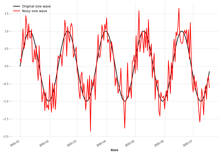
We create a simple sine wave signal and add Gaussian noise to it.

NOISE_DISTANCE = 0.4
SAMPLE_SIZE = 200
np.random.seed(42)

# Prepare the sine wave
x = tg.sine_timeseries(length=SAMPLE_SIZE, value_frequency=0.025)

# Add white noise
noise = tg.gaussian_timeseries(length=SAMPLE_SIZE, std=NOISE_DISTANCE)
x_noise = x + noise

plt.figure(figsize=[12, 8])
x.plot(label="Original sine wave")
x_noise.plot(color="red", label="Noisy sine wave")
plt.legend()
plt.show()

Infer the mean of a Gaussian Process using a periodic kernel

Next, we fit a Gaussian Process on the data using the ExpSineSquared kernel. This kernel encodes a periodicity assumption, which is appropriate for our data. You can try to uncomment the kernel = RBF() line to change the kernel to an RBF kernel, which only imposes smoothness of the function. See The Kernel Cookbook for more information about (Gaussian Process) kernels and how to combine them.

The GaussianProcessFilter constructor takes the same arguments as scikit-learn’s GaussianProcessRegressor on which is relies. The kernels implemented in scikit-learn can be found here.

Here, we set a relative noise variance of alpha=0.2 because we know exactly how much noise we added before, but in practice this will have to estimated.

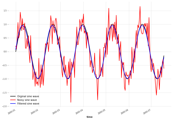
We see that the mean of Gaussian Process lies very close to the original signal. Bear in mind though that real data will rarely be so perfectly periodic and more experimentation with kernels and noise levels will be needed.

kernel = ExpSineSquared()
# kernel = RBF()

gpf = GaussianProcessFilter(
    kernel=kernel, alpha=NOISE_DISTANCE / 2, n_restarts_optimizer=100
)
filtered_x = gpf.filter(x_noise)

plt.figure(figsize=[12, 8])
x.plot(color="black", label="Orginal sine wave")
x_noise.plot(color="red", label="Noisy sine wave")
filtered_x.plot(color="blue", label="Filtered sine wave")
plt.legend()

<matplotlib.legend.Legend at 0x166c993a0>

Sample from a Gaussian Process

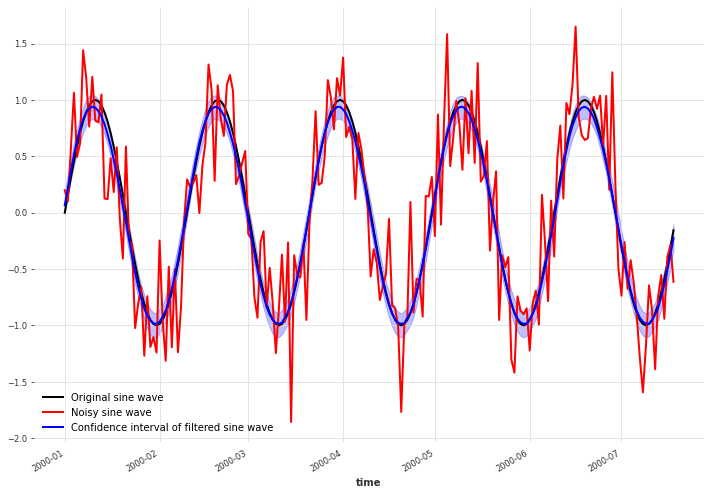
The Gaussian Process is a probabilistic model, meaning that the predictions of the model are distributions instead of single values.

Before, we just used the mean of these distributions at the points of interest to plot a curve. Here instead, we will sample from the distributions and plot the 90% confidence interval. From this we can see that the uncertainty about the underlying data is larger around the crests and troughs than elsewhere.

filtered_x_samples = gpf.filter(x_noise, num_samples=100)

plt.figure(figsize=[12, 8])
x.plot(color="black", label="Original sine wave")
x_noise.plot(color="red", label="Noisy sine wave")
filtered_x_samples.plot(color="blue", label="Confidence interval of filtered sine wave")
plt.legend()

<matplotlib.legend.Legend at 0x166b2eca0>

Sample from a Gaussian Process with missing data points

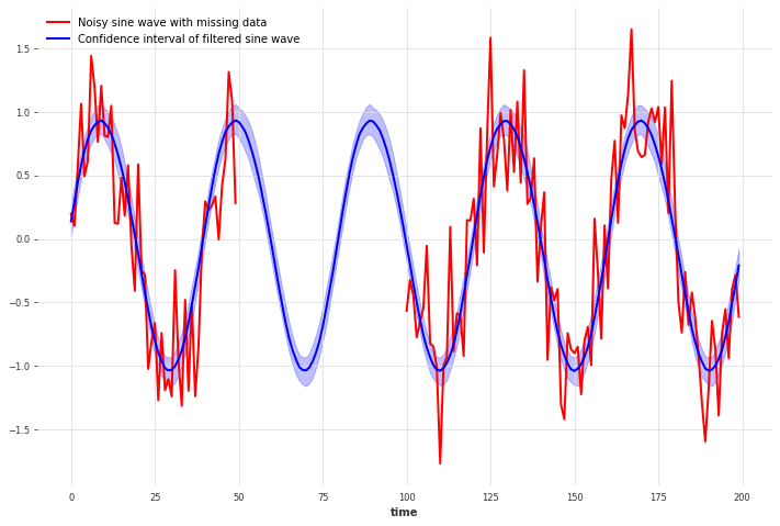
We can even use the Gaussian Process filter on time series with missing (NaN) data points.

For our periodic signal, the Gaussian Process estimates the missing data very well using the periodic kernel. You can see how this changes and the uncertainty increases when using the RBF kernel instead.

x_missing_arr = x_noise.values()
x_missing_arr[50:100] = np.nan
x_missing = TimeSeries.from_values(x_missing_arr)

kernel = ExpSineSquared()
# kernel = RBF()

gpf_missing = GaussianProcessFilter(kernel=kernel, alpha=0.2, n_restarts_optimizer=100)
filtered_x_missing_samples = gpf_missing.filter(x_missing, num_samples=100)

plt.figure(figsize=[12, 8])
x_missing.plot(color="red", label="Noisy sine wave with missing data")
filtered_x_missing_samples.plot(
    color="blue", label="Confidence interval of filtered sine wave"
)
plt.legend()

<matplotlib.legend.Legend at 0x166db4a00>

previous

Filtering and predicting using the darts filters

next

Dynamic Time Warping (DTW)