Ensembling Models#
The following is a brief demonstration of the ensemble models in Darts. Starting from the examples provided in the Quickstart Notebook, some advanced features and subtilities will be detailed.
The following topics are covered in this notebook :
[1]:
# fix python path if working locally
from utils import fix_pythonpath_if_working_locally

fix_pythonpath_if_working_locally()
[2]:
%load_ext autoreload
%autoreload 2
%matplotlib inline
import warnings

import matplotlib.pyplot as plt

# use darts plotting style
from darts import set_option

set_option("plotting.use_darts_style", True)

from darts.dataprocessing.transformers import Scaler
from darts.datasets import AirPassengersDataset
from darts.metrics import mape
from darts.models import (
    ExponentialSmoothing,
    KalmanForecaster,
    LinearRegressionModel,
    NaiveDrift,
    NaiveEnsembleModel,
    NaiveSeasonal,
    RandomForestModel,
    RegressionEnsembleModel,
    TCNModel,
)
from darts.utils.timeseries_generation import (
    datetime_attribute_timeseries as dt_attr,
)

warnings.filterwarnings("ignore")

import logging

logging.disable(logging.CRITICAL)
Basics & references#
Ensembling combines the forecasts of several “weak” models to obtain a more robust and accurate model.
All of Darts’ ensembling models rely on the stacking technique (reference). They provide the same functionalities as the other forecasting models. Depending on the ensembled models, they can:
levarage covariates
be trained on multiple-series
predict multivariate targets
generate probabilistic forecasts
and more…
[3]:
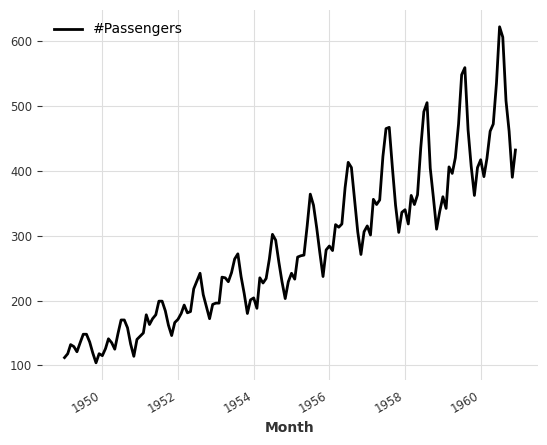
# using the AirPassenger dataset, directly available in darts
ts_air = AirPassengersDataset().load()
ts_air.plot()
[3]:
<Axes: xlabel='Month'>
Naive Ensembling#
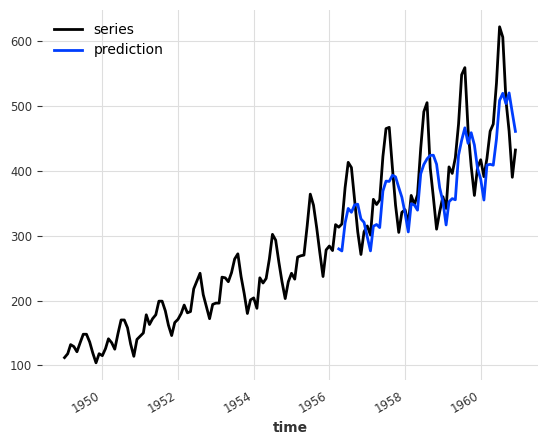
Naive ensembling simply takes the average (mean) of the forecasts generated by the ensembled forecasting models. Darts’ NaiveEnsembleModel accepts both local and global forecasting models (as well as combination of the two, with some additional limitations).
[4]:
naive_ensemble = NaiveEnsembleModel(
    forecasting_models=[NaiveSeasonal(K=12), NaiveDrift()]
)

backtest = naive_ensemble.historical_forecasts(ts_air, start=0.6, forecast_horizon=3)

ts_air.plot(label="series")
backtest.plot(label="prediction")
print("NaiveEnsemble (naive) MAPE:", round(mape(backtest, ts_air), 5))
NaiveEnsemble (naive) MAPE: 11.87818
Note: after looking at the each model’s MAPE, one would notice that NaiveSeasonal is actually performing better on its own than ensembled with NaiveDrift. Checking the performance of the single models is in general a good practice before defining an ensemble.
Before creating the new NaiveEnsemble, we will screen models to identify which ones would do well together. The candidates are :
LinearRegressionModel: classic and simple modelExponentialSmoothing: moving window modelKalmanForecaster: a filter-based modelRandomForestModel: decision trees model
[5]:
candidates_models = {
    "LinearRegression": (LinearRegressionModel, {"lags": 12}),
    "ExponentialSmoothing": (ExponentialSmoothing, {}),
    "KalmanForecaster": (KalmanForecaster, {"dim_x": 12}),
    "RandomForestModel": (RandomForestModel, {"lags": 12, "random_state": 0}),
}

backtest_models = []

for model_name, (model_cls, model_kwargs) in candidates_models.items():
    model = model_cls(**model_kwargs)
    backtest_models.append(
        model.historical_forecasts(ts_air, start=0.6, forecast_horizon=3)
    )
    print(f"{model_name} MAPE: {round(mape(backtest_models[-1], ts_air), 5)}")
LinearRegression MAPE: 4.64008
ExponentialSmoothing MAPE: 4.44774
KalmanForecaster MAPE: 4.5539
RandomForestModel MAPE: 8.02264
[6]:
fix, axes = plt.subplots(2, 2, figsize=(9, 6))
for ax, backtest, model_name in zip(
    axes.flatten(),
    backtest_models,
    list(candidates_models.keys()),
):
    ts_air[-len(backtest) :].plot(ax=ax, label="ground truth")
    backtest.plot(ax=ax, label=model_name)

    ax.set_title(model_name)
    ax.set_ylim([250, 650])
plt.tight_layout()
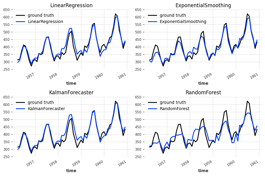
The historical forecasts obtained with the LinearRegressionModel and KalmanForecaster look quite similar whereas ExponentialSmoothing tends to understimate the true values and RandomForestModel is failing to capture the peaks. To benefits from the ensemble, we will favor diversity and continue with the LinearRegressionModel and ExponentialSmoothing.£
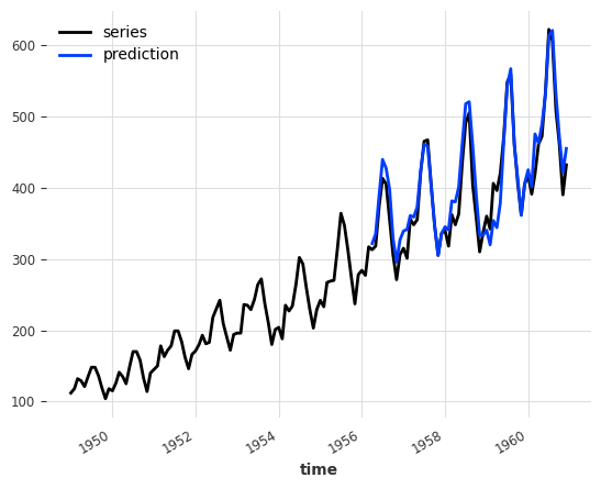
[7]:
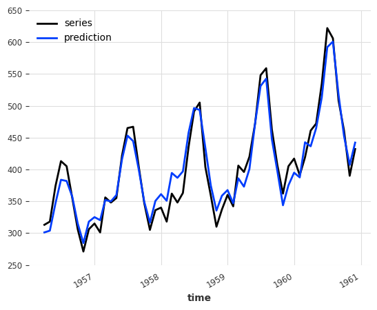
ensemble = NaiveEnsembleModel(
    forecasting_models=[LinearRegressionModel(lags=12), ExponentialSmoothing()]
)

backtest = ensemble.historical_forecasts(ts_air, start=0.6, forecast_horizon=3)

ts_air[-len(backtest) :].plot(label="series")
backtest.plot(label="prediction")
plt.ylim([250, 650])
print("NaiveEnsemble (v2) MAPE:", round(mape(backtest, ts_air), 5))
NaiveEnsemble (v2) MAPE: 4.04297

Compared to the individual model MAPE score, 4.64008 for the LinearRegressionModel and 4.44874 for the ExponentialSmoothing, the ensembling improved the accuracy to 4.04297!
Using covariates & predicting multivariate series#
Depending on the forecasting models used, the EnsembleModel can of course also leverage covariates or forecast multivariates series! The covariates will be passed only to the forecasting models supporting them.
In the example below, the ExponentialSmoothing model does not support any covariates whereas the LinearRegressionModel model supports future_covariates.
[8]:
ensemble = NaiveEnsembleModel([
    LinearRegressionModel(lags=12, lags_future_covariates=[0]),
    ExponentialSmoothing(),
])

# encoding the months as integer, normalised
future_cov = dt_attr(ts_air.time_index, "month", add_length=12) / 12
backtest = ensemble.historical_forecasts(
    ts_air, future_covariates=future_cov, start=0.6, forecast_horizon=3
)

ts_air[-len(backtest) :].plot(label="series")
backtest.plot(label="prediction")
plt.ylim([250, 650])
print("NaiveEnsemble (w/ future covariates) MAPE:", round(mape(backtest, ts_air), 5))
NaiveEnsemble (w/ future covariates) MAPE: 4.07502
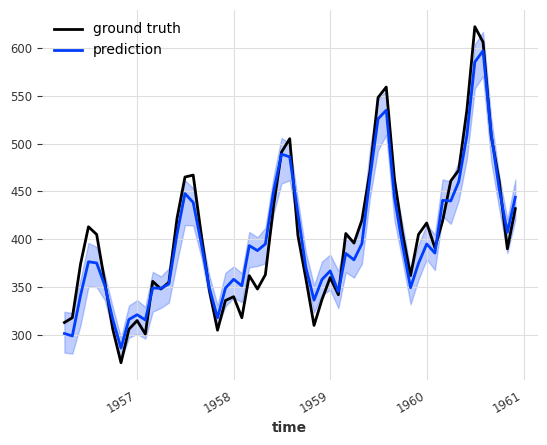
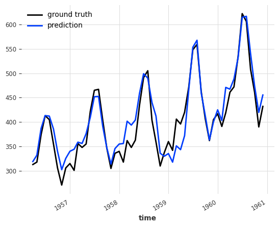
Probabilistic naive ensembling#
Combining models supporting probabilistic forecasts results in a probabilistic NaiveEnsembleModel! We can easily tweak the models used above to make them probabilistic and obtain confidence interval in ours forecasts:
[9]:
ensemble_probabilistic = NaiveEnsembleModel(
    forecasting_models=[
        LinearRegressionModel(
            lags=12,
            likelihood="quantile",
            quantiles=[0.05, 0.5, 0.95],
        ),
        ExponentialSmoothing(),
    ]
)

# must pass num_samples > 1 to obtain a probabilistic forecasts
backtest = ensemble_probabilistic.historical_forecasts(
    ts_air, start=0.6, forecast_horizon=3, num_samples=100
)

ts_air[-len(backtest) :].plot(label="ground truth")
backtest.plot(label="prediction")
[9]:
<Axes: xlabel='time'>
Learned Ensembling#
Ensembling can also be considered as a supervised regression problem: given a set of forecasts (features), find a model that combines them in order to minimise errors on the target. This is what the RegressionEnsembleModel does. The main three parameters are:
forecasting_modelsis a list of forecasting models whose predictions we want to ensemble.regression_train_n_pointsis the number of time steps to use for fitting the “ensemble regression” model (i.e., the inner model that combines the forecasts).regression_modelis, optionally, a sklearn-compatible regression model or a DartsSKLearnModelto be used for the ensemble regression. If not specified, Darts’LinearRegressionModelis used. Using a sklearn model is easy out-of-the-box, but using one of Darts’ regression models allows to potentially take arbitrary lags of the individual forecasts as inputs of the regression model.
Once these elements are in place, a RegressionEnsembleModel can be used like a regular forecasting model:
[10]:
ensemble_model = RegressionEnsembleModel(
    forecasting_models=[NaiveSeasonal(K=12), NaiveDrift()],
    regression_train_n_points=12,
)

backtest = ensemble_model.historical_forecasts(ts_air, start=0.6, forecast_horizon=3)

ts_air.plot()
backtest.plot()

print("RegressionEnsemble (naive) MAPE:", round(mape(backtest, ts_air), 5))
RegressionEnsemble (naive) MAPE: 4.85142
Compared to the MAPE of 11.87818 obtained at the beginning of the naive ensembling section, adding a LinearRegressionModel on top of the two naive models does improve the quality of the forecast.
Now, let’s see if we can observe similar gain when the RegressionEnsemble forecasting models are not naive:
[11]:
ensemble = RegressionEnsembleModel(
    forecasting_models=[LinearRegressionModel(lags=12), ExponentialSmoothing()],
    regression_train_n_points=12,
)

backtest = ensemble.historical_forecasts(ts_air, start=0.6, forecast_horizon=3)

ts_air.plot(label="series")
backtest.plot(label="prediction")

print("RegressionEnsemble (v2) MAPE:", round(mape(backtest, ts_air), 5))
RegressionEnsemble (v2) MAPE: 4.63334
Interestingly, even if the MAPE improved compared to the RegressionEnsemble relying on naive models (MAPE: 4.85142), it does not outperform the NaiveEnsemble using similar forecasting models (MAPE: 4.04297).
This performance gap is partially caused by the points set aside to train the ensembling LinearRegression; the two forecasting models (LinearRegression and ExponentialSmoothing) cannot access the latest values of the series, which contains a marked upward trend.
Out of curiosity, we can use the Ridge regression model from the sklearn library to ensemble the forecasts:
[12]:
from sklearn.linear_model import Ridge

ensemble = RegressionEnsembleModel(
    forecasting_models=[LinearRegressionModel(lags=12), ExponentialSmoothing()],
    regression_train_n_points=12,
    regression_model=Ridge(),
)

backtest = ensemble.historical_forecasts(ts_air, start=0.6, forecast_horizon=3)

print("RegressionEnsemble (Ridge) MAPE:", round(mape(backtest, ts_air), 5))
RegressionEnsemble (Ridge) MAPE: 6.46803
In this particuliar scenario, using a regression model with a regularization term deteriorated the forecasts but there might be other cases where it will improve them.
Training using historical forecasts#
When predicting a number of values greater than their output_chunk_length, GlobalForecastingModels rely on auto-regression (use their own output as input) to forecast values far in the future. However, the quality of the forecasts can considerably decrease as the predicted timestamp get further from the end of the observations. During RegressionEnsemble’s regression model training, the forecasting models generate forecasts for timestamps where the ground truth is actually known and
available, making it possible to use historical_forecasts instead of predict().
This can be activated with train_using_historical_forecasts=True.
Under the hood, the ensemble model will trigger historical forecasting for each model with forecast_horizon=model.output_chunk_length, stride=model.output_chunk_length, last_points_only=False, and overlap_end=False to predict the last regression_train_n_points points of the target series.
[ ]:
# replacing the ExponentialSmoothing (local) with RandomForestModel (global)
ensemble = RegressionEnsembleModel(
    forecasting_models=[
        LinearRegressionModel(lags=12),
        RandomForestModel(lags=12, random_state=0),
    ],
    regression_train_n_points=12,
    train_using_historical_forecasts=False,
)
backtest = ensemble.historical_forecasts(ts_air, start=0.6, forecast_horizon=3)

ensemble_hist_fct = RegressionEnsembleModel(
    forecasting_models=[
        LinearRegressionModel(lags=12),
        RandomForestModel(lags=12, random_state=0),
    ],
    regression_train_n_points=12,
    train_using_historical_forecasts=True,
)
backtest_hist_fct = ensemble_hist_fct.historical_forecasts(
    ts_air, start=0.6, forecast_horizon=3
)

print("RegressionEnsemble (no hist_fct) MAPE:", round(mape(backtest, ts_air), 5))
print("RegressionEnsemble (hist_fct) MAPE:", round(mape(backtest_hist_fct, ts_air), 5))
RegressionEnsemble (no hist_fct) MAPE: 5.7016
RegressionEnsemble (hist_fct) MAPE: 5.12017
As expected, using historical forecasts with the forecasting models to the train the regression model produces better forecasts.
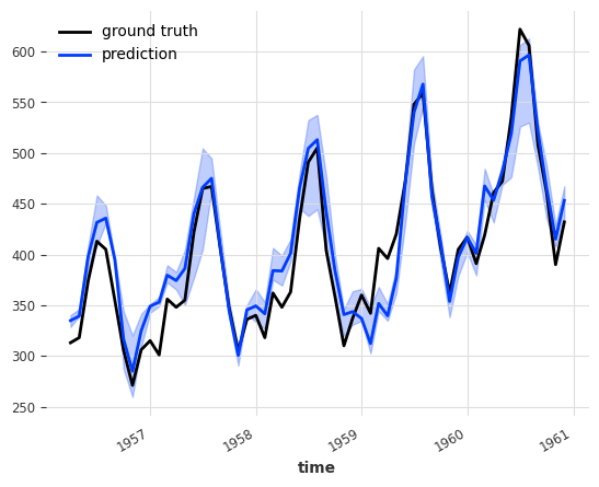
Probabilistic regression ensemble#
In order to be probabilistic, the RegressionEnsembleModel, must have a probabilistic ensembling regression model (see table in the README):
[14]:
ensemble = RegressionEnsembleModel(
    forecasting_models=[LinearRegressionModel(lags=12), ExponentialSmoothing()],
    regression_train_n_points=12,
    regression_model=LinearRegressionModel(
        lags_future_covariates=[0], likelihood="quantile", quantiles=[0.05, 0.5, 0.95]
    ),
)

backtest = ensemble.historical_forecasts(
    ts_air, start=0.6, forecast_horizon=3, num_samples=100
)

ts_air[-len(backtest) :].plot(label="ground truth")
backtest.plot(label="prediction")

print("RegressionEnsemble (probabilistic) MAPE:", round(mape(backtest, ts_air), 5))
RegressionEnsemble (probabilistic) MAPE: 5.15071
Bootstrapping regression ensemble#
When the forecasting models of a RegressionEnsembleModel are probabilistic, the samples dimension of their forecasts is reduced and used as covariates for the ensembling regression. Since the ensembling regression model is deterministic, the generated forecasts is deterministic as well.
[15]:
ensemble = RegressionEnsembleModel(
    forecasting_models=[
        LinearRegressionModel(
            lags=12, likelihood="quantile", quantiles=[0.05, 0.5, 0.95]
        ),
        ExponentialSmoothing(),
    ],
    regression_train_n_points=12,
    regression_train_num_samples=100,
    regression_train_samples_reduction="median",
)

backtest = ensemble.historical_forecasts(ts_air, start=0.6, forecast_horizon=3)

ts_air[-len(backtest) :].plot(label="ground truth")
backtest.plot(label="prediction")

print("RegressionEnsemble (bootstrap) MAPE:", round(mape(backtest, ts_air), 5))
RegressionEnsemble (bootstrap) MAPE: 5.10138
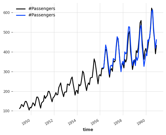
Pre-trained Ensembling#
As both NaiveEnsembleModel and RegressionEnsembleModel accept GlobalForecastingModel as forecasting models, they can be used to ensemble pre-trained deep learning and regression models. Note that this functionnality is only supported if all the ensembled forecasting models are instances from the GlobalForecastingModel class and are already trained when creating the ensemble.
Disclaimer : Be careful not to pre-train the models with data used during validation as this would introduce considerable bias.
Note : The parameters for the TCNModel is heavily inspired from the TCNModel example notebook.
[16]:
# holding out values for validation
train, val = ts_air.split_after(0.8)

# scaling the target
scaler = Scaler()
train = scaler.fit_transform(train)
val = scaler.transform(val)

# use the month as a covariate
month_series = dt_attr(ts_air.time_index, attribute="month", one_hot=True)
scaler_month = Scaler()
month_series = scaler_month.fit_transform(month_series)

# training a regular linear regression, without any covariates
linreg_model = LinearRegressionModel(lags=24)
linreg_model.fit(train)

# instanciating a TCN model with parameters optimized for the AirPassenger dataset
tcn_model = TCNModel(
    input_chunk_length=24,
    output_chunk_length=12,
    n_epochs=500,
    dilation_base=2,
    weight_norm=True,
    kernel_size=5,
    num_filters=3,
    random_state=0,
)
tcn_model.fit(train, past_covariates=month_series)
[16]:
TCNModel(kernel_size=5, num_filters=3, num_layers=None, dilation_base=2, weight_norm=True, dropout=0.2, input_chunk_length=24, output_chunk_length=12, n_epochs=500, random_state=0)
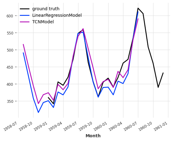
As a sanity check, we will look at the forecast of the model taken individually:
[17]:
# individual model forecasts
pred_linreg = linreg_model.predict(24)
pred_tcn = tcn_model.predict(24, verbose=False)

# scaling them back
pred_linreg_rescaled = scaler.inverse_transform(pred_linreg)
pred_tcn_rescaled = scaler.inverse_transform(pred_tcn)

# plotting
ts_air[-24:].plot(label="ground truth")
pred_linreg_rescaled.plot(label="LinearRegressionModel")
pred_tcn_rescaled.plot(label="TCNModel")
plt.show()
Now that we have a good idea of the individual performance of each of these models, we can ensemble them. We must make sure to set train_forecasting_models=False or the ensemble will need to be fitted before being able to call predict().
Advice : Use the save() method to export your model and keep a copy of your weights.
[18]:
naive_ensemble = NaiveEnsembleModel(
    forecasting_models=[tcn_model, linreg_model], train_forecasting_models=False
)
# NaiveEnsemble initialized with pre-trained models can call predict() directly,
# the `series` argument must however be provided
pred_naive = naive_ensemble.predict(len(val), train)

pretrain_ensemble = RegressionEnsembleModel(
    forecasting_models=[tcn_model, linreg_model],
    regression_train_n_points=24,
    train_forecasting_models=False,
    train_using_historical_forecasts=False,
)
# RegressionEnsemble must train the ensemble model, even if the forecasting models are already trained
pretrain_ensemble.fit(train)
pred_ens = pretrain_ensemble.predict(len(val))

# scaling back the predictions
pred_naive_rescaled = scaler.inverse_transform(pred_naive)
pred_ens_rescaled = scaler.inverse_transform(pred_ens)

# plotting
plt.figure(figsize=(8, 5))
scaler.inverse_transform(val).plot(label="ground truth")
pred_naive_rescaled.plot(label="pre-trained NaiveEnsemble")
pred_ens_rescaled.plot(label="pre-trained RegressionEnsemble")
plt.ylim([250, 650])

# MAPE
print("LinearRegression MAPE:", round(mape(pred_linreg_rescaled, ts_air), 5))
print("TCNModel MAPE:", round(mape(pred_tcn_rescaled, ts_air), 5))
print("NaiveEnsemble (pre-trained) MAPE:", round(mape(pred_naive_rescaled, ts_air), 5))
print(
    "RegressionEnsemble (pre-trained) MAPE:", round(mape(pred_ens_rescaled, ts_air), 5)
)
LinearRegression MAPE: 3.91311
TCNModel MAPE: 4.70491
NaiveEnsemble (pre-trained) MAPE: 3.82837
RegressionEnsemble (pre-trained) MAPE: 3.61749
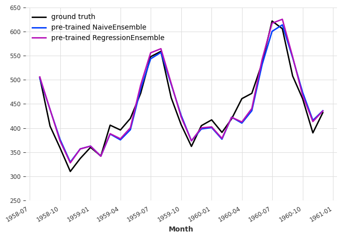
Conclusion#
Ensembling pre-trained LinearRegression and TCNModel models allowed us to out-perform single models and training a linear regression on top of these two models forecasts further improved the MAPE score.
If the gains remain limited on this small dataset, ensembling is a powerful technique that can yield impressive results and was notably used by the winners of the 4th edition of the Makridakis Competition (website, github repository).