Foundation Models

In this notebook, we will show how to use time series foundation models in Darts. If you are new to Darts, please check out the Quickstart Guide before proceeding.

Foundation models are pre-trained on large-scale time series data and can be used for zero-shot forecasting – that means they can produce forecasts without any training or fine-tuning. Darts currently supports the following foundation models:

• Chronos2Model – Amazon’s Chronos-2 (paper, blog)

• TimesFM2p5Model – Google’s TimesFM 2.5 (paper)

• TiRexModel – NX-AI’s TiRex (paper)

All models support the following:

• uni- and multivariate time series

• single and multiple time series

• deterministic and probabilistic forecasting

• zero-shot forecasting

• fine-tuning

They differ in covariate support and installation requirements:

Model	Past Covariates	Future Covariates	Static Covariates	Extra Dependency
Chronos2Model	✅	✅	🔴
TimesFM2p5Model	🔴	🔴	🔴
TiRexModel	🔴	🔴	🔴	tirex-ts>=1.4.0

This notebook demonstrates common usage patterns with Chronos2Model. Other foundation models can be used in exactly the same way – the only differences are covariate support (see table above) and installation requirements.

# fix python path if working locally
from utils import fix_pythonpath_if_working_locally

fix_pythonpath_if_working_locally()
%matplotlib inline

%load_ext autoreload
%autoreload 2
%matplotlib inline

# use darts plotting style
from darts import set_option

set_option("plotting.use_darts_style", True)

import warnings

import numpy as np

from darts.datasets import ElectricityConsumptionZurichDataset
from darts.metrics import mae, mic, miw
from darts.models import Chronos2Model

# Other foundation models can be imported in the same way:
# from darts.models import TimesFM2p5Model
# from darts.models import TiRexModel  # requires: pip install tirex-ts>=1.4.0
from darts.utils.likelihood_models import QuantileRegression

warnings.filterwarnings("ignore")
import logging

logging.disable(logging.CRITICAL)

Data Preparation

Here, we will use the Electricity Consumption Zurich Dataset, which records the electricity consumption of households & SMEs ("Value_NE5" column) and business & services ("Value_NE7") in Zurich, Switzerland, along with weather covariates such as temperature ("T [°C]") and humidity ("Hr [%Hr]"). Values are recorded every 15 minutes between January 2015 and August 2022.

Train-Test Split

Even though foundation models are pre-trained already, we still need to split the data into training and test sets. That is because they follow the Darts unified interface and will require calling the fit() method before forecasting. However, no training or fine-tuning will be performed during the fit() call.

Data Scaling

Unlike other deep learning models in Darts, foundation models do not require data scaling since they have their own internal data normalization mechanism. Therefore, we will skip the scaling step in this notebook.

# convert to float32
data = ElectricityConsumptionZurichDataset().load().astype(np.float32)
# extract households energy consumption
ts_energy = data["Value_NE5"]
# extract temperature, solar irradiation and rain duration
ts_weather = data[["T [°C]", "StrGlo [W/m2]", "RainDur [min]"]]
# split into train and validation sets by last 7 days
train_energy, val_energy = ts_energy.split_before(len(ts_energy) - 7 * 24 * 4)

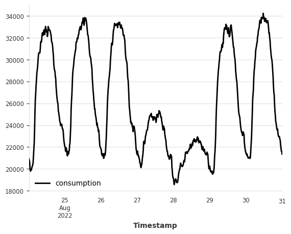
Let’s quickly visualize the last 7 days of the electricity consumption data.

val_energy.plot(label="consumption");

Model Creation

In the following, we demonstrate model creation using Chronos2Model. The same pattern applies to other foundation models – simply swap the model class.

All foundation models support two types of forecasting outputs:

• Deterministic forecasts (default): single point estimates for each future time step.

• Probabilistic forecasts: multiple samples for each future time step, which can be used to estimate prediction intervals. To enable probabilistic forecasting, set likelihood=QuantileRegression([...]) when creating the model. The list of quantiles used here must be a subset of the model’s supported quantiles. For Chronos-2: [0.01, 0.05, 0.1, 0.15, 0.2, 0.25, 0.3, 0.35, 0.4, 0.45, 0.5, 0.55, 0.6, 0.65, 0.7, 0.75, 0.8, 0.85, 0.9, 0.95, 0.99].

Lookback and Forward Windows

Under the hood, foundation models are no different from other Torch Forecasting Models (TFMs) in Darts and most hyperparameters from TFMs can be applied here as well. In particular, you can control the length of the lookback window and the forward window using the input_chunk_length and output_chunk_length parameters, respectively.

• input_chunk_length: the number of time steps of history the model takes as input when making a forecast. Maximum is 8192 for Chronos-2.

• output_chunk_length: the number of time steps the model outputs in one forward pass. If the forecast horizon is longer than this value, the model consumes its own previous predictions to produce further forecasts. This is known as the autoregressive forecasting. Maximum is 1024 for Chronos-2.

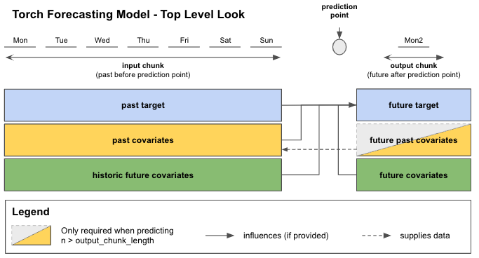
See the Torch Forecasting Models User Guide for more details.

Model Downloading and Caching

When creating a foundation model instance for the first time, the pre-trained model checkpoint will be automatically downloaded from Hugging Face Hub and cached locally. Subsequent usage will NOT re-download the files but use the cached version instead.

If you would like to download or load the model checkpoint to a custom directory, set local_dir argument when creating the model. For example:

model = Chronos2Model(
    input_chunk_length=168,
    output_chunk_length=24,
    local_dir="path/to/your/directory"
)

Using Smaller or Synthetic Variants (Chronos-2)

Two variants of Chronos-2 are available on HuggingFace Hub:

• autogluon/chronos-2-small : a smaller 28M parameter Chronos-2 model.

• autogluon/chronos-2-synth : a 120M parameter Chronos-2 model trained on synthetic data only.

To use either of those variants, specify the hub_model_name parameter to the desired model ID. For example, to use the synthetic data variant:

model = Chronos2Model(
    input_chunk_length=168,
    output_chunk_length=24,
    hub_model_name="autogluon/chronos-2-small",
    hub_model_revision=None, # e.g., branch, tag, or commit ID
)

# use last 30 days of data to predict next 7 days
model = Chronos2Model(
    input_chunk_length=30 * 24 * 4,
    output_chunk_length=7 * 24 * 4,
)

Model Training

Here, we will call the fit() method to “train” the model on the training set. Note that no actual training or fine-tuning will be performed since foundation models are already pre-trained.

model.fit(
    series=train_energy,
    verbose=True,
)

Chronos2Model(output_chunk_shift=0, likelihood=None, hub_model_name=amazon/chronos-2, hub_model_revision=None, local_dir=None, input_chunk_length=2880, output_chunk_length=672)

Forecasting

We now perform a one-shot forecast for the next 7 days. We then compare the forecast against the actual values from the validation set.

pred = model.predict(
    n=7 * 24 * 4,
    series=train_energy,
)
val_energy.plot(label="actual")
pred.plot(label="forecast");

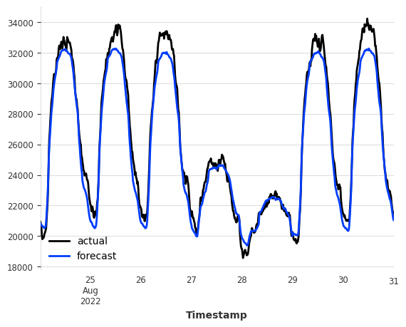
You can see that the model is able to produce qualitatively accurate forecasts without any training or fine-tuning! Let’s evaluate the forecast accuracy using the Mean Absolute Error (MAE) metric.

mae_val = mae(val_energy, pred)
print(f"MAE on validation set: {mae_val:.2f}")

MAE on validation set: 653.57

Model Fine Tuning

Fine-tuning can be enabled via the enable_finetuning model creation parameter. You can find detailed examples in our fine-tuning examples.

Forecasting with Covariates

This section only applies to foundation models that support covariates (such as Chronos2Model).

Recall that Chronos-2 supports forecasting with covariates (exogenous variables). Since no training is required, we do not worry about hyperparameter tuning for covariates. Forecasting with covariates is as simple as passing the covariate series to the fit() and predict() methods!

We use weather variables as future covariates to help forecast the electricity consumption. We then compare the forecast (with and without covariates) against the actual values from the validation set.

The weather variables here are actual measurements from a weather station and not forecasts (not actual future covariates). The results shown here for demonstration purposes only. In practice, you should supply weather forecasts as future covariates to get realistic results.

model = Chronos2Model(
    input_chunk_length=30 * 24 * 4,
    output_chunk_length=7 * 24 * 4,
)
model.fit(
    series=train_energy,
    future_covariates=ts_weather,
    verbose=True,
)
pred_cov = model.predict(
    n=7 * 24 * 4,
    series=train_energy,
    future_covariates=ts_weather,
)
val_energy.plot(label="actual")
pred_cov.plot(label="forecast with covariates")
pred.plot(label="forecast without covariates");

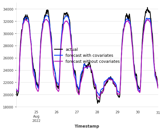
With future covariates such as weather, we see that the forecast accuracy has improved on the 7-day horizon! Covariate support from Chronos-2 can be very useful when exogenous variables have a strong influence on the target series.

mae_cov = mae(val_energy, pred_cov)
print(f"MAE on validation set with covariates: {mae_cov:.2f}")

MAE on validation set with covariates: 466.05

Probabilistic Forecasting

All foundation models support probabilistic forecasting. Here, we show how to perform probabilistic forecasting using QuantileRegression likelihood. The quantiles passed to QuantileRegression must be a subset of the model’s pre-trained quantiles (see “Model Creation” section above for Chronos-2).

Because sampling with large foundation models can be computationally expensive, we here call predict() with predict_likelihood_parameters=True to obtain quantile estimates directly without sampling. However, if the forecast horizon is longer than output_chunk_length (i.e., auto-regressive forecasting is required), you must call predict() with a large enough num_samples value (e.g., 1000) to generate probabilistic forecasts via Monte Carlo sampling.

model = Chronos2Model(
    input_chunk_length=30 * 24 * 4,
    output_chunk_length=7 * 24 * 4,
    likelihood=QuantileRegression(quantiles=[0.1, 0.5, 0.9]),
)
model.fit(
    series=train_energy,
    future_covariates=ts_weather,
    verbose=True,
)
pred_prob = model.predict(
    n=7 * 24 * 4,
    series=train_energy,
    future_covariates=ts_weather,
    predict_likelihood_parameters=True,
)
val_energy.plot(label="actual")
pred_prob.plot(label="forecast");

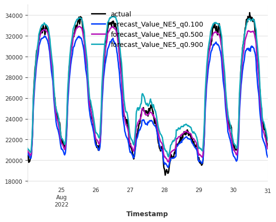
For probabilistic forecasts, we can evaluate the forecast quality by computing the Mean Interval Coverage (MIC) (the share of actuals inside the prediction intervals) and Mean Interval Width (MIW) (the width of the prediction intervals) metrics to evaluate the quality of the prediction intervals.

For MIC, we expect a value close to the nominal coverage of the prediction intervals (i.e., 80% for the (0.1, 0.9) interval). For MIW, lower values indicate narrower prediction intervals and thus better forecast quality when MIC is satisfactory.

mic_prob = mic(val_energy, pred_prob, q_interval=(0.1, 0.9))
miw_prob = miw(val_energy, pred_prob, q_interval=(0.1, 0.9))
print(f"MIC on validation set with covariates: {mic_prob:.2%}")
print(f"MIW on validation set with covariates: {miw_prob:.2f}")

MIC on validation set with covariates: 82.74%
MIW on validation set with covariates: 1719.57

Final Remarks

Just like other Torch Forecasting Models in Darts, foundation models support historical forecasting (historical_forecasts()), backtesting (backtest()), residual computation (residuals()), custom PyTorch Lightning arguments (pl_trainer_kwargs), and more. Check out the following resources to learn more about those topics:

• Torch Forecasting Models User Guide

• Fine Tuning Examples

• Using Torch Models with GPUs and TPUs

• Backtesting: simulate historical forecasting

• Chronos2Model API

• TimesFM2p5Model API

• TiRexModel API